In order to analyze chaos in a simple system, we will consider the
basic equation, called after the German engineer and freelance
researcher Georg Wilhelm Christian Caspar Duffing
(1861--1944). Duffing had a heart valve defect that freed him from military service.
The Duffing equation was originally derived as a model for describing the forced vibrations of inductrial machinery. It provides a very good approximation of the motion of a damped, driven inverted pendilum with a torsional restoring force. The unforced pendulum equation is
\[
m \ell^2 \ddot{\theta} + mg\ell \,\sin \theta + \gamma \dot{\theta} + k\theta
=0,
\]
where θ is the angle of inclinantion of the bob of mass
m from the downward vertical position,
k is the torsional spring constant, and γ is the damping coefficient. Here dot denotes the derivative with respect to time
t (Newton's notation). Upon approximation the sine function by its two term Maclausin polynomial, we get
\[
\ddot{\theta} + \frac{g}{\ell}\left[ \theta - \frac{1}{6}\,\theta^3 \right] + \gamma \dot{\theta} + k\theta
=0,
\]
where we keep the same notations for coefficients
k and γ. Linear terms can be united.
Nowadays, the term "Duffing equation" is used for any equation that
describes an oscillator that has a cubic stiffness term, regardless of
the type of damping or excitation.
\begin{equation} \label{EqDuffing.1}
\ddot{x} + \gamma \,\dot{x} + \omega_0^2 x + \beta\,x^3 =0 .
\end{equation}
This, however, was not the case in Duffing’s original work. The above
equation can display chaotic behavior. For ω
0²>0, the
Duffing oscillator can be interpreted as a forced oscillator with a spring
whose restoring force is written as
F = - ω
0²
x - β
x3. When β>0, this equation
represents a "hard spring," and for β<0, it represents a "soft
spring." If β<0, the phase portrait curves are closed.
We analyze the unforced system first.
For ω0²<0 (so ω0 is pure imaginary),
the Duffing oscillator describes the dynamics of a point mass in a double well
potential, and it can be regarded as a model of a periodically forced steel
beam which is deflected toward the two magnets. It is known that chaotic
motions can be observed in this case.
When there is no resistance proportional to the velocity (γ = 0), the
Duffing equation can be integrated upon multiplication by the velocity:
\[
\dot{x} \left( \ddot{x} + \omega_0^2 x + \beta\,x^3 \right) =
\frac{\text d}{{\text d}t} \left( \frac{1}{2}\, \dot{x}^2 +
\frac{1}{2}\,\omega_0^2 x^2 + \frac{1}{4}\, \beta\,x^4 \right) = 0.
\]
Integration yields
\[
E(t) = \frac{1}{2}\, \dot{x}^2 + \frac{1}{2}\,\omega_0^2 x^2 +
\frac{1}{4}\, \beta\,x^4 = \mbox{constant} .
\]
The function in parenthesis
\( H= \frac{1}{2}\, \dot{x}^2 +
\frac{1}{2}\,\omega_0^2 x^2 + \frac{1}{4}\, \beta\,x^4 \) is called
the
Hamiltonian for the Duffing equation. Then
\[
\dot{x} = \frac{\partial H}{\partial y} , \qquad \dot{y} = -
\frac{\partial H}{\partial x} .
\]
For positive coefficients ω²
0 and β, the solution
is bounded:
\( |x| \le \sqrt{2H/\omega_0^2} \) and
\( |\dot{x}| \le \sqrt{2H} . \)
When γ≥0, the function
E(t) satisfies
\[
\frac{{\text d}E(t)}{{\text d}t} = - \gamma\,\dot{x}^2 \le 0;
\]
therefore,
E(t) is a Lyapunov function, and every trajectory moves on
the surface of
E(t) toward the equilibrium position---the origin. When
the Duffing equation has nonzero coefficients, there exist stationary
solutions that are obtained upon solving the cubic equation
\[
\omega_0^2 x + \beta\,x^3 =0 \qquad \mbox{or} \qquad x \left( \omega_0^2 +
\beta\,x^2 \right) =0 .
\]
So we get two other equilibrium solutions
\( x =
\pm \sqrt{- \omega_0^2 / \beta} , \) when
\(
\omega_0^2 \beta < 0 . \) To analyze their stability, we apply
the linearization procedure, so we calculate the Jacobian matrix
\[
{\bf J} (x) = \begin{bmatrix} 0&1 \\ - \omega_0^2 - 3\beta\, x^2 & -\gamma
\end{bmatrix} .
\]
The eigenvalues of
J(0) are
\[
\lambda = -\frac{1}{2} \left[ \gamma \pm \sqrt{\gamma^2 - 4\omega_0^2} \right] ,
\]
and it is found that this equilibrium is stable for
\(
\omega_0^2 \ge 0 . \) On the other hand, the eigenvalues of the
equilibria
\( x = \pm \sqrt{- \omega_0^2 /\beta} \)
are
\[
\lambda = -\frac{1}{2} \left[ \gamma \pm \sqrt{\gamma^2 + 8\omega_0^2} \right] ,
\]
which are unstable for positive values of γ and ω
0.
We are going to find the general solution to Duffing’s equation
\[
\ddot{x} + \omega_0^2 x + \beta\,x^3 =0
\]
in terms of
the
Jacobi
elliptic function cn, called the elliptic cosine. This
function is defined as follows:
\[
\mbox{cn} (t,k) = \cos \phi , \quad \mbox{where} \quad t =
\int_0^{\phi} \frac{{\text d}\theta}{\sqrt{1- k^2 \sin^2 \theta}} .
\]
Elliptic functions are functions of two variables. The first variable
might be given in terms of the
amplitude φ. The second variable might
be given in terms of the parameter
m, or as the elliptic
modulus
k, where
k² =
m, or in terms of the
modular angle α, where
m = sin² α. Out of twelve Jacobi
elliptic functions, there are two other elliptic functions closely
related to the previous one: the elliptic sine
sn and the delta amplitude
dn. They are
defined by
\[
\mbox{sn} (t,k) = \sin \phi \quad \mbox{and} \quad \mbox{dn}(t,k) =
\sqrt{1- k^2 \sin^2 \phi} .
\]
Mathematica has build-in corresponding
functions:
JacobiSN,
JacobiCN, and
JacobiDN.
The number
m =
k² (0 <
m < 1)
is called elliptic modulus and the number φ is
called Jacobi amplitude and it is denoted by am(
t,
m).
The following identities are hold:
\[
\mbox{sn}^2 (t,k) + \mbox{cn}^2 (t,k) =1, \quad \mbox{dn}^2 (t,k) = 1
- k^2 \mbox{sn}^2 (t,k) .
\]
Since elliptic functions satisfy the following differential equations
\[
\frac{\text d}{{\text d}t}\,\mbox{sn}(t,k) =
\mbox{cn}(t,k)\,\mbox{dn}(t,k), \quad
\frac{\text d}{{\text d}t}\,\mbox{cn}(t,k) =
\mbox{sn}(t,k)\,\mbox{dn}(t,k), \quad
\frac{\text d}{{\text d}t}\,\mbox{dn}(t,k) = - k^2
\mbox{sn}(t,k)\,\mbox{cn}(t,k),
\]
it can be shown that the function
\( x = c_1
\mbox{cn}(\omega t + c_2 , k) \) satisfies following
differential equation
\[
\ddot{x} + \omega^2 \left( 1 - 2 k^2 \right) x(t) + \frac{2k^2
\omega^2}{c_1^2} \, x^3 (t) =0 ,
\]
for any constants
c1
and
c2. Therefore, the general solution to Duffing's
equation is obtained by solving the system
\[
\omega_0^2 = \omega^2 \left( 1 - 2 k^2 \right) , \qquad \beta = \frac{2k^2
\omega^2}{c_1^2}
\]
which gives
\[
\omega = \sqrt{\omega_0^2 + c_1^2 \beta} , \qquad k =
\sqrt{\frac{c_1^2 \beta}{2 \left(
\omega_0^2 + c_1^2 \beta \right)}} .
\]
So we proved that the solution to the initial value problem
\[
\ddot{x} + \omega_0^2 x + \beta\,x^3 =0 , \qquad x(0) = x_0 , \quad
\dot{x} (0) = x_1
\]
is
\[
x(t) = c_1 \mbox{cn}\left( \sqrt{\omega_0^2 + c_1^2 \beta}\, t + c_2 ,\
\sqrt{\frac{c_1^2 \beta}{2 \left(
\omega_0^2 + c_1^2 \beta \right)}} \right) ,\qquad \omega_0^2 + c_1^2 \beta
\ne 0,
\]
where the values of
c1
and
c2 are determined from the initial conditions. If
x1 = 0, then
c1 =
x0 and
c2 = 0, so
\[
x(t) = x_0 \mbox{cn}\left( \sqrt{\omega_0^2 + x_0^2 \beta}\, t , \
\sqrt{\frac{x_0^2 \beta}{2 \left(
\omega_0^2 + x_0^2 \beta \right)}} \right) ,\qquad \omega_0^2 + x_0^2 \beta
\ne 0 .
\]
This solution is periodic and bounded if
\( \omega_0^2 +
\beta\,x_0^2 > 0 \) for any β. In case when
\( \omega_0^2 +
\beta\,x_0^2 < 0 , \) solutions are bounded when β > 0;
other wise, they are unbounded.
When the initial displacement is zero, x0 = 0 but
the velocity is not x1 ≠ 0, the solution of the Duffing
equation is expressed via elliptic sine function because it is a solution of
the second order differential equation:
\[
\frac{{\text d}^2}{{\text d}u^2}\,\mbox{sn}(u,k) + \left( 1 + k \right)
\mbox{sn}(u,k) - 2k^2 \mbox{sn}^3 (u,k) = 0 , \qquad \mbox{sn}(0,k) = 0, \quad
\left. \frac{\text d}{{\text d}u}\, \mbox{sn}(u,k) \right\vert_{u=0} =
\left. \mbox{cn}(u,k)\,\mbox{dn}(u,k)\right\vert_{u=0} =1.
\]
Some particular cases:
-
The solution to the initial value problem
\[
\ddot{x} + x - \frac{1}{6}\, x^3 =0 , \qquad x(0) =0, \quad \dot{x} (0) =1 ,
\]
is
\[
x(t) = \frac{1}{\lambda}\,\mbox{sn}(\lambda t, k) , \qquad \lambda =
\frac{3 + \sqrt{6}}{6} \approx 9.89898, \quad k^2 =
\frac{1- \lambda^2}{\lambda^2} \approx 0.101021.
\]
-
The solution to the initial value problem
\[
\ddot{x} + 2\,x +2\, x^3 =0 , \qquad x(0) =1, \quad \dot{x} (0) =0 ,
\]
is
\[
x(t) = \mbox{cn}(2t, 1/2) .
\]
This solution is bounded and periodic with period 2K(1/2) ≈
3.3715, where K is the complete elliptic integral
of the first kind: \( \displaystyle K(m) = \int_0^{\pi /2}
\frac{{\text d}\phi}{\sqrt{1 - m\, \sin^2 \phi}} = \int_0^1 \left( 1 - s^2 \right){-1/2} \left( 1 - m \,s^2 \right){-1/2} {\text d}s . \)
-
The solution to the initial value problem
\[
\ddot{x} - 2\,x - 2\, x^3 =0 , \qquad x(0) =1, \quad \dot{x} (0) =0 ,
\]
is
\[
x(t) = \mbox{cn} \left( 2 \sqrt{-1}\,t, 1/2 \right) = \mbox{nc} \left( 2t,
\sqrt{3}/2 \right) .
\]
This solution is unbounded and periodic with period 2K(3½/2) ≈ 4.313.
Here Jacobi elliptic function nc has default notation in Mathematica
as JacobiNC.
-
The initial value problem
\[
\ddot{x} +x - 2\, x^3 =0 , \qquad x(0) =1, \quad \dot{x} (0) =0 ,
\]
has unbounded and periodic solution x(t) = sec(t).
-
The initial value problem
\[
\ddot{x} +3\,x - x^3 =0 , \qquad x(0) =2, \quad \dot{x} (0) =0 ,
\]
has unbounded and periodic solution with period 4K(2-1/2)/2
≈ 5.2441
\[
x(t) = 2\,\mbox{dc} \left( \sqrt{2}\,t , 1/\sqrt{2} \right) .
\]
-
The initial value problem
\[
\ddot{x} +2\,x - x^3 =0 , \qquad x(0) =1, \quad \dot{x} (0) =0 ,
\]
has unbounded and periodic solution with period 4K(3-1/2)/2
≈ 8.0086
\[
x(t) = 2\,\mbox{cd} \left( \sqrt{3/2}\,t , 1/\sqrt{3} \right) .
\]
-
The initial value problem
\[
\ddot{x} -2\,x + 13\, x^3 =0 , \qquad x(0) =1, \quad \dot{x} (0) =0 ,
\]
has bounded and periodic solution with period
\[
x(t) = ????
\]
-
■
close all
clear all
clc

global delta alpha beta gamma omega

delta = 0.3;
alpha = -1;
beta  = 1;
omega = 1.2;

length = 400;
maxx = 1000;

for i = 1:length
    gamma = i/10;

    [t(i,:), x(i,:,:)] = ode45(@(t,x) duff(t,x,delta,alpha,beta,gamma,omega), ...
        0:2*pi/omega/100:(maxx*2*pi/omega/100), [0 1]);
end

for i = 1:length

    figure(1)

    t0 = t(i,:);
    x0 = x(i,:,1);

    plot(t0(100:maxx-100), x0(100:maxx-100), 'color', '#D95319', 'LineWidth', 1.5)
    title(sprintf('Time Series at γ = %.2f\n', i/20))
    ylim([-10 10])
    xlim([10 40])

    pause(0.05)
end

for i = 1:length

    figure(2)

    x1 = x(i,:,1);
    x2 = x(i,:,2);

    plot(x2(100:maxx-100), x1(100:maxx-100), 'color', '#0072BD', 'LineWidth', 1)
    title(sprintf('Phase Space at γ = %.2f\n', i/20))
    ylim([-12, 12])
    xlim([-6, 6])

    pause(0.05)
end

function xdot = duff(t,x,delta,alpha,beta,gamma,omega)

xdot(1) = -delta*x(1)+alpha*x(2)-beta*x(2)^3+gamma*cos(omega*t);
xdot(2) = x(1);
xdot = xdot';
end
|
|
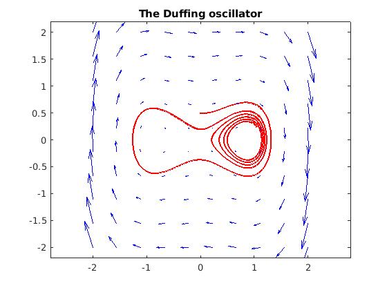
d = 0.04; a = 1; b = -.75;
F = chebfun2v(@(x,y)y, @(x,y) -d*y - b*x - a*x.^3, [-2 2 -2 2]);
[t y] = ode45(F,[0 40],[0,0.5]);
plot(y,'r','LineWidth',2), hold on
quiver(F,'b'), axis equal
title('The Duffing oscillator'), hold off
|
|
Duffing oscillator.
|
|
Chebfun code
|
d = 0.04; a = 1; b = -.75;
F = chebfun2v(@(x,y)y, @(x,y) -d*y - b*x - a*x.^3, [-2 2 -2 2]);
[t y] = ode45(F,[0 40],[0,0.5]);
plot(y,'r'), hold on
quiver(F,'b'), axis equal
title('The Duffing oscillator'), hold off