Suppose that you want to investigate the performance of a feedback controller that is
intended to hold a quadcopter at a prescribed altitude
We assume that the
quadcopter moves only vertically. Magnitude of the lift force (which comes from four engines, in newtons) is given by
are 3 constants that can be tuned to give the best performance of the system. We use the following notations:
\( t \) is time (in seconds);
\( v_y \) is vertical speed (meters per second) of vehicle;
\( L \) is length of rotor blades (in meters);
\( \rho = 1.2 \,\mbox{kg/m}^2\) -- air density;
\( P(t) = k_p \,e(t) + k_d \,\frac{{\text d}\,e}{{\text d}\,t} + k_i \,\int e(t)\,{\text d}t \) is power (in watts) of one of four motors;
\( k_p, \ k_d , \ k_i \) -- constants;
\( F_d = c\, v^2 \) is drag force (in newtons), where c is a constant;
\( e= h-y \) is an error;
\( h \) is an altitude.
So basically engine power \( P(t) \) is input, and \( h \) is a given attitude. Now we write the system of differential equations:
\[
\begin{split}
\frac{{\text d}y}{{\text d} t} &= v_y , \\
\frac{{\text d} v_y}{{\text d} t} &= \frac{8\,P}{\left( v_y m +C \right)} - \frac{c\,v_y^2}{m} -g , \\
\frac{{\text d}Q}{{\text d} t} &= h-y ,
\end{split}
\]
where \( C = 2m \,\sqrt{\frac{mg}{\pi \rho L^2}} . \) To solve this system of equations,
we introduce the vector of three unknowns: \( {\bf w} = \langle y, v_y , Q \rangle^T \) (T stands for transposition).
Then its derivative is
\[
\frac{{\text d}{\bf w}}{{\text d} t} = \left[ \begin{array}{c} {\text d}y/{\text d}t \\ {\text d}v_y /{\text d}t
\\ {\text d}Q /{\text d}t \end{array} \right] = \frac{{\text d}}{{\text d} t} \left[ \begin{array}{c} y \\ v_y \\ Q \end{array} \right] ,
\]
which we denote as dwdt in Matlab code. We solve this system of equations numerically using the following numerical values:
	function helicopter
clear all;
% Below are the given constants
m=10/1000;% mass is actually 10 grams
L=2/100;  % length of the rotor blades in cm
c=0.0012; % constant number
p=1.2;    % air density in kg/m^3
g=9.8;    % gravity acceleration in m/sec^2
dhdt=0;   % fixed altitude
h=1;      % height
initial_condition1=[0;0;0]; %y=vy=Q=0

% write ode45 functions and plot
% under 1st set of Kp, Kd, Ki constants
Kp=1; Kd=0; Ki=0; % chosen Kp, Kd, Ki constants
[times_1,sols_1] = ode45(@helicopter, [0:0.1:20], initial_condition1);
figure
hold on
plot(times_1,sols_1(:,1),'LineWidth',2,'Color',[1,0,0])
ylabel('h (m)','Fontsize',16);
xlabel('time (s)','Fontsize',16);
title(('Height of Helicopter'),'Fontsize',20);

% under 2nd set of Kp, Kd, Ki constants
initial_condition2=[0;0;0];
Kp=1; Kd=0.2; Ki=0;
[times_2,sols_2] = ode45(@helicopter, [0:0.1:20], initial_condition2);
plot(times_2,sols_2(:,1),'LineWidth',2,'Color',[0,1,0])

% under 3rd set of Kp, Kd, Ki constants
initial_condition3=[0;0;0];
Kp=1; Kd=0.2; Ki=0.2;
[times_3,sols_3] = ode45(@helicopter, [0:0.1:20], initial_condition3);
plot(times_3,sols_3(:,1),'LineWidth',2,'Color',[0,0,1])
legend('K parameters1','K parameters2','K parameters3')

%solve for the height of the helicopter given different parameters and test
%the performance of the controller
    function dwdt = helicopter(t,w)
        y = w(1); vy=w(2); Q=w(3);
        dydt=vy; %vertical speed
        dvydt=8*(Kp*(h-y)+Kd*(dhdt-dydt)+Ki*Q)/(vy*m+2*m*sqrt(m*g/(pi*p*L^2)))-(c*vy^2/m)-g; %plug P(t) into FL
        dQdt=h-y; %accounts for error
        dwdt=[dydt;dvydt;dQdt];
end
end
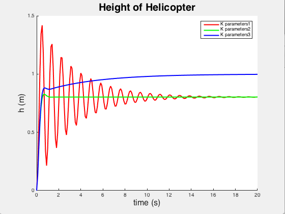
In the problem, the unknown functions \( y, \ v_y , \ Q \) are denoted by
\( w(1), \,w(2), \, w(3) ,\) respectively. From the graph, we see that the third set of parameters
\( k_p ,\, k_d , \,k_i \) controls the system with greater precision.
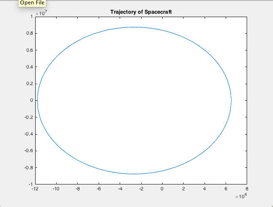
Example 2.3.2: Spacecraft
The lending motion of a spacecraft is modeled by the following system of differential equations
\[
\begin{split}
\frac{{\text d}R}{{\text d}t} &= v_r ,
\\
\frac{{\text d}\theta}{{\text d}t} &= \omega ,
\\
\frac{{\text d}v_r}{{\text d}t} &= -B + R\,\omega^2 -C\,v_r ,
\\
\frac{{\text d}\omega}{{\text d}t} &= - \frac{2\,v_r \omega}{R} - C\,\omega ,
\end{split}
\]
where
\[
B= g\,\frac{R^2_e}{R^2} , \qquad C= \frac{1}{2m}\, \rho_0 C_d \,A\,v_r \,e^{\left( -\frac{R-R_e}{d} \right)} , \qquad v= \sqrt{v_r^2 + \left( R\omega \right)^2} .
\]
Here
\( \rho = \rho_0 \,e^{-h/d} \) is air density;
\( {\bf F}_d = - \frac{1}{2}\,\rho\,C_d A\,v\,{\bf v} \) is drag force,
\( v = \sqrt{v_r^2 + (R\omega )^2} \) is speed,
\( A \) is area of front,
\( C_d \) is drag coefficient,
\( {\bf F}_g = -mg\,\frac{R_e^2}{R^2}\,{\bf r} \) is gravitational force,
h is the distance above earth,
\( R \) is magnitude of position vector {\bf R},
\( R_e \) is radius of the earth.
We denote the unknow functions as \( R= w(1), \ \theta = w(2), \ v_r = w(3) .\) The initial conditions are as follows:
\( R= R_e + h_0 ,\)
\( \theta_0 =0 ,\)
\( v_r = v_0 \sin \phi , \)
\( \omega = v_0 \cos \phi /R ;\)
here \( \phi \) is re-entry angle, \( h_0 = 122\,\mbox{km} \) is the re-entry altitude. It is convenient to introduce the polar coordinates:
\[
x= R\,\cos\theta , \qquad y=R\,\sin\theta .
\]
function capsule ??? to be modified
%% Problem 2
% We want to compute the trajectory of a spacecraft during reentry into the
% earth's atmosphere. Air density is given by p = po*e^(-h/d). Drag force
% is given by Fd = -1/2p*Cd*A*V. The gravitational force is given by Fg =
% -m*g*(Re^2/R^3). Use differential equations to relate R and theta and
% their time derivatives and solve for the trajectory of the spacecraft.

% Declare constants
m=8600;       % capsule mass in kg
A=2.5^2*pi;   % diameter of heat shield pi*r^2 in meters
Cd=0;         % drag coefficient
Re=6371*1000; % earth radius in m
d=5*1000;     % density decay length in m
p0=1.2;       % air density at sea level in kg/hr
h0=122*1000;  % re-entry altitude in meters
V0=32000*(1000/3600); % velocity at re-entry
g=9.8;        % gravity acceleration
phi=0;        % re-entry angle
options = odeset('Event',@event_function2,'RelTol',0.000001);
initial_condition = [Re+h0; 0; -V0*sin(phi); V0*cos(phi)/(Re+h0)]; %provide initial conditions
[times,sols] = ode45(@spacecraft,[0,(240*60)],initial_condition,options);

% write function to solve the trajectory of the spacecraft
    function dwdt = spacecraft(t,w)
        R = w(1); theta=w(2); vR=w(3); omega= w(4);
        v=sqrt(vR^2+(R*omega)^2);
        dRdt = vR;  dthetadt=omega;
        dvRdt = -g*(Re^2/R^2) + R*(omega^2) - (((1/2)*p0*Cd*A*v)/m)*exp(-(R-Re)/d)*vR;
        domegadt = (-(2*vR*omega)/(R))-((1/2)*(p0*Cd*A*v/m)*exp(-(R-Re)/d))*omega;
        dwdt = [dRdt;dthetadt;dvRdt;domegadt];
end
 function [val,stop,dir] = event_function2(t,w)
        R = w(1); theta=w(2); vR=w(3); omega = w(4);
        val = R-Re;
        stop = 1;   % this stops matlab when the spacecraft hits the ground
        dir = -1; % interested in y crossing zero from positive to negative
 end

for i=1:length(times)
    x(i) = sols(i,1)*cos(sols(i,2));
    y(i) = sols(i,1)*sin(sols(i,2));
end
% plot the spacecraft's trajectory
figure
plot(x,y)
title('Trajectory of Spacecraft')
end
Example 2.3.3: Lorenz Attractor
We will wrap up this series of examples with a look at the fascinating Lorenz Attractor. The Lorenz system is a system of ordinary differential equations
(the Lorenz equations, note it is not Lorentz) first studied by the professor of MIT Edward Lorenz (1917--2008) in 1963. It is notable for having chaotic solutions
for certain parameter values and initial conditions. In particular, the Lorenz attractor is a set of chaotic solutions of the Lorenz system which, when plotted,
\[
\begin{split}
\frac{{\text d}x}{{\text d}t} &= \sigma\left( y-x \right) ,
\\
\frac{{\text d}y}{{\text d}t} &= x \left( \rho -z \right) -y,
\\
\frac{{\text d}z}{{\text d}t} &= x\, y - \beta \, z .
\end{split}
\]
The equations are made up of three populations: x, y, and z, and three fixed coefficients: \( \sigma ,\ \rho , \mbox{ and } \ \beta .\)
Remembering what we discussed previously, this system of equations has properties common to most other complex systems, such as lasers, dynamos, thermosyphons, brushless DC motors, electric circuits, and chemical reactions. First, it is non-linear in two places:
the second equation has a xz term and the third equation has a xy term. It is made up of a very few simple components. The system is three-dimensional and deterministic. Although difficult to see until we plot
the solution, the equation displays broken symmetry on multiple scales. Because the equation is autonomous (no t term in the right side of the equations),
there is no feedback in this case.
This system’s behavior depends on the three constant values chosen for the coefficients. It has been shown that the Lorenz System exhibits complex behavior
when the coefficients have the following specific values: \( \sigma = 10, \ \rho = 28 , \mbox{ and }\ \beta = 8/3. \)
We now have everything we need to code up the ODE into Matlab. However, we will write two codes, one we call attractor.m, and another one is lorenz.m.
We now have everything we need to code up the ODE into Matlab.
function attractor
% The Lorenz strange attractor
% Implements the Lorenz System ODE
% dx/dt = sigma*(y-x)
% dy/dt = x*(rho-z)-y
% dz/dt = xy-beta*z%
% Inputs:
% ~ - time variable: the name is not used here because system is autonomous.
% Y - dependent variable: has 3 dimensions
% Output:
% dYdt - First derivative: the rate of change of the three dimension
% values over time, given the values of each dimension
t0=0; % Initial point
tn=20; % Terminal point
Y0=[10, 10, 10]; % Initial values
% Standard constants for the Lorenz Strange Attractor
sigma = 10;
rho = 28;
beta = 8/3;
[t, Y] = ode45(@ lorenz, [t0, tn], Y0); % RelTol 1e-3 (default)
% Create 3d Plot
figure('name','The Lorenz strange attractor')
plot3(Y(:,1), Y(:,2), Y(:,3));
grid
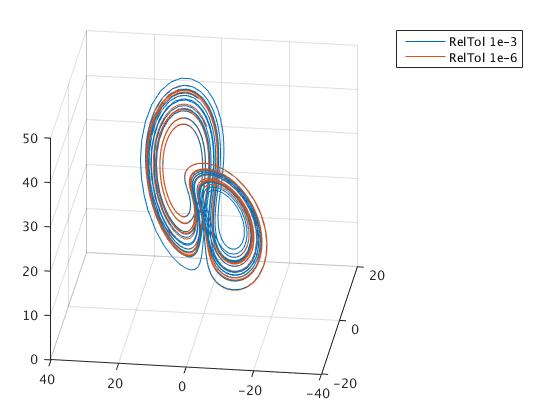
[t1,Y1] = ode45(@ lorenz, [t0, tn], Y0, odeset('RelTol', 1e-6));
figure('Name','The Lorenz strange attractor, comparison')
plot3(Y(:,1),Y(:,2),Y(:,3), Y1(:,1),Y1(:,2),Y1(:,3))
legend('RelTol 1e-3','RelTol 1e-6')
grid
figure('Name',...
'The Lorenz strange attractor, RelTol 1e-3 (blue) and 1e-6 (red)')
subplot(3, 1, 1)
plot(t,Y(:,1), t1,Y1(:,1))
ylabel('x')
subplot(3, 1, 2)
plot(t,Y(:,2),t1,Y1(:,2))
ylabel('y')
subplot(3, 1, 3)
plot(t,Y(:,3), t1,Y1(:,3))
ylabel('z')
xlabel('t')
disp('Numbers of steps for RelTol 1e-3 and 1e-6')
disp([numel(t),numel(t1)])
function dYdt = lorenz(~,X)
% The Lorenz strange attractor
dxdt = sigma*(X(2)-X(1));
dydt = X(1)*(rho-X(3))-X(2);
dzdt = X(1)*X(2)-beta*X(3);
dYdt = [dxdt; dydt; dzdt];
end
end
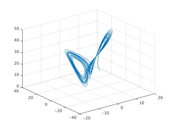
The output consists of the following graphs:
and three solutions for \( x(t),\ y(t) \) , and \( z(t) \) , respectively:
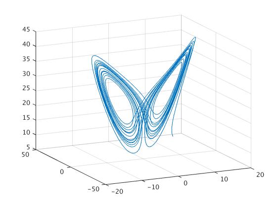
Matlab allow you to rotate the picture: just click on the icon and drag the cursor. You will get another view of the pictures:
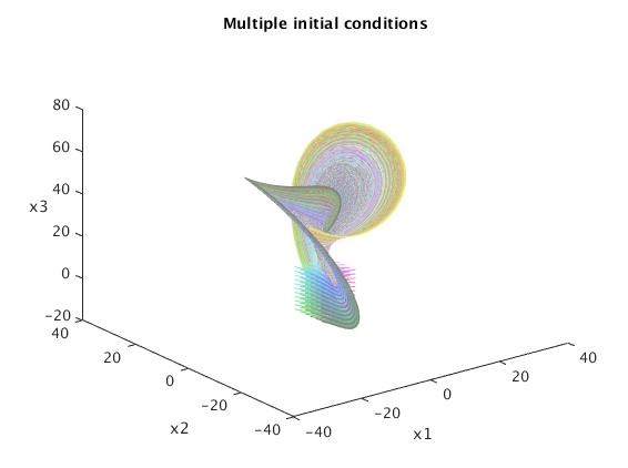
I have picked a starting point of [10 10 10] and I encourage you to play around with other starting points. Because this is a system of three equations, the solution can be plotted in three dimensions. Because the shape of the solution is somewhat complex, we can use “rotation” icon of tool bar and rotate 3D plot.
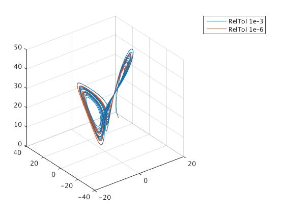
It turns out that Matlab allows you to choose how forgiving you want your solver to be. You can set the relative error tolerance (‘RelTol’) and the absolute error tolerance (‘AbsTol’). I simply changed the relative error tolerance. The default relative error tolerance is 0.001. I lowered a value of that tolerance down to 1e-6 (it means did a tolerance higher) and compared the two solutions. In the following examples, the red solution is generated using the 1e-6 relative tolerance. We set the error tolerance using the odeset function. Then we evaluate the solutions while passing in the returned value from the odeset function. Make note that in this example, the two solutions are using the exact same set of equations and starting at the exact same point.
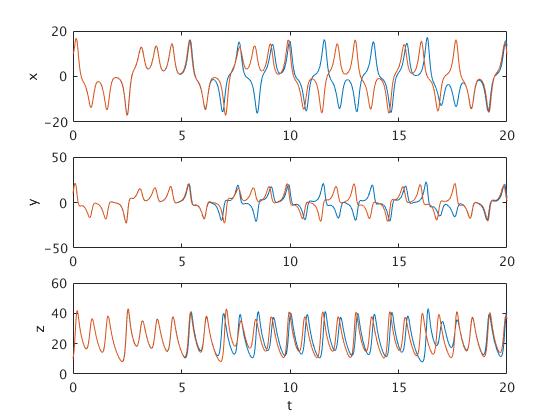
As you can see, the two solutions do seem to diverge. You can see it somewhat clearly in the inner part of the orbits, where one shows mostly blue and the other red. Still, it’s tricky to see exactly how quickly and where the two diverge. To get a better look at it, we splitted the 3D graph into three separate graphs, one for each dimension.
Keep in mind that this is the exact same graph as the previous figure, just plotted differently. Here we can indeed see that the two solutions diverge very rapidly (although rapidly may be a misnomer as we are ignoring units in this lesson). Blue and red seem to diverge somewhere between time 5 and 10, and while they do come back into close proximity, they never join back together (just like our logistic map example).
How did this difference happen? Recall what I said about how a higher error tolerance forces the numerical solver to take smaller steps. In each case, the solver went from time 0 to time 20. But, let’s see how many steps each took to get there. We printed these quantities
>> attractor
Numbers of steps for RelTol 1e-3 and 1e-6
        1233        4389
Thus, the same solver, solving the same equation, starting at the same starting point, took over 3.5 times more steps than the default approach when using a higher error tolerance. Furthermore, not only did it take more steps and presumably generate a more accurate solution, after a short period of similarity, the more accurate solver generated a completely different solution than the default solver! The interesting question is to ask, how quickly did our `good’ solver diverge from the real solution? It should be to always question the results of your numerical solutions to ODEs that describe complex and/or chaotic systems. It only takes small missteps for your solution to rapidly diverge from the actual solution.
We present another version solving Lorenz equations numerically and plotting the results. This includes several steps.
Step 1. Define an anonymous function, or save it as a separate function file. We write three dots in order to prolong the command.
mylorenz = @(x,sigma,rho,beta)...
[ sigma * (x(2) - x(1)); ...
rho * x(1)-x(1) * x(3) - x(2); ...
x(1) * x(2) - beta * x(3) ];
Step 2. Specify the parameters and define an anonymous function that
can be used by an ODE solver.
sigma = 10; beta = 8/3; rho = 30;
lorenzxdot = @(t,x) mylorenz(x,sigma,rho,beta);
Note:These two lines above need to be run each time when any of the parameters is changed.
Step 3. Choose initial values and a time interval for the solution and compute an approximate using a built-in Runge–Kutta solver.
x0 = [3;4;1];
Tmax = 40;
[time,solvec] = ode45(lorenzxdot, [0,Tmax],x0);
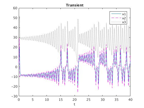
The solutions can then be plotted next to each other or in a three-dimensional plot.
figure
plot(time,solvec(:,1),'-',time,solvec(:,2),'m--',time,solvec(:,3),'k:')
legend('x1','x2','x3')
title('Transient')
xlabel('t')
% Will plot x(1) and x(2) as a function of time on the same graph.
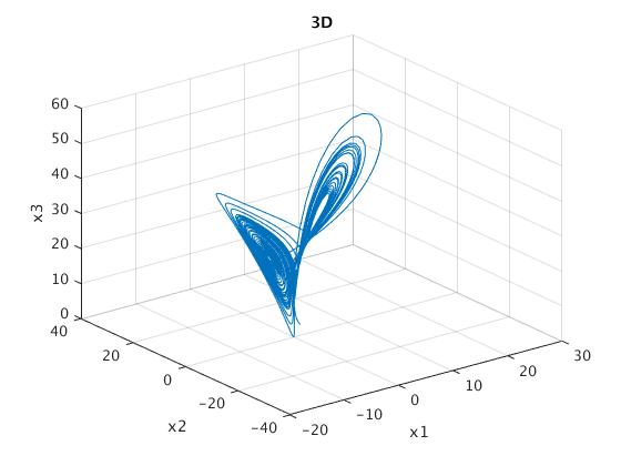
figure
plot3(solvec(:,1),solvec(:,2),solvec(:,3))
xlabel('x1')
ylabel('x2')
zlabel('x3')
title('3D')
grid on
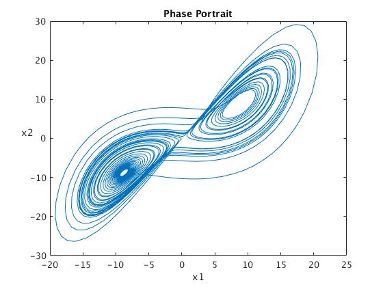
While the following will be a plot in the phase plane for x(1) and x(2):
figure
plot(solvec(:,1),solvec(:,2))
xlabel('x1')
ylabel('x2','rotation',0)
title('Phase Portrait')
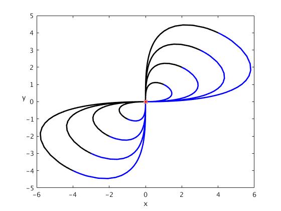
% Multiple Initial Conditions
x1_0 = -5:2:5;
y1_0 = -5:2:5;
z1_0 = -10:2:10;
Tmax = 10;
figure
view(3);
title('Multiple initial conditions')
xlabel('x1')
ylabel('x2')
zlabel('x3','rotation',0)
hold on
for i = 1:numel(x1_0)
  for j = 1:numel(y1_0)
    for k = 1:numel(z1_0)
      x0 = [x1_0(i);y1_0(j);z1_0(k)];
      [time,solvec] = ode45(lorenzxdot, [0,Tmax],x0);
      plot3(solvec(:,1),solvec(:,2),solvec(:,3),'Color',...
        [(-min(x1_0) + i)/(2*numel(x1_0)), (-min(y1_0) +j)/...
        (2*numel(y1_0)), (-min(z1_0) + k)/(2*numel(z1_0))]) %fun colors
      drawnow
    end
  end
end
hold off
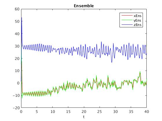
Ensemble
In order to simulate the Lorenz equations for an ensemble of initial
data, define the functions mylorenz and lorenzxdot as above, together
with suitable choices for the parameters sigma, beta, rho.
Let Tmax be the length of the time interval, and let N be the ensemble
size (the number of simulations). The following code computes the means
of N with initial data x0 + xi , where xi is a normal random vector with
zero mean and standard deviation gamma.
N = 10;
gamma = .5;
Tmax = 40;
x0 = [3;15;1];
tt = linspace(0,Tmax,10*Tmax);
xEns = 0*tt;
yEns = 0*tt;
zEns = 0*tt;
for j = 1:N
[t,solvec] = ode45(lorenzxdot, [0,Tmax],x0 + gamma*randn(3,1));
% tt corresponds to the points of interpolation;
xEns = xEns + spline(t,solvec(:,1),tt);
yEns = yEns + spline(t,solvec(:,2),tt);
zEns = zEns + spline(t,solvec(:,3),tt);
end
xEns = xEns/N;
yEns = yEns/N;
zEns = zEns/N;

figure
plot(tt,xEns,'r',tt,yEns,'g',tt,zEns,'b')
legend('xEns','yEns','zEns')
title('Ensemble')
xlabel('t')
xEns = xEns + interp1(t,solvec(:,1),tt);
yEns = yEns + interp1(t,solvec(:,2),tt);
zEns = zEns + interp1(t,solvec(:,3),tt);
In dynamical systems, a first recurrence map or Poincaré map, named after Henri Poincaré, is the intersection of a periodic orbit in the state space of a continuous dynamical system with a certain lower-dimensional subspace, called the Poincaré section, transversal to the flow of the system. More precisely, one considers a periodic orbit with initial conditions within a section of the space, which leaves that section afterwards, and observes the point at which this orbit first returns to the section. One then creates a map to send the first point to the second, hence the name first recurrence map. The transversality of the Poincaré section means that periodic orbits starting on the subspace flow through it and not parallel to it.
A Poincaré map can be interpreted as a discrete dynamical system with a state space that is one dimension smaller than the original continuous dynamical system. Because it preserves many properties of periodic and quasiperiodic orbits of the original system and has a lower-dimensional state space, it is often used for analyzing the original system in a simpler way. In practice this is not always possible as there is no general method to construct a Poincaré map.
In the
Poincaré section method
one records the coordinates of a trajectory
whenever the trajectory crosses a prescribed trigger. This
triggering event can be
as simple as vanishing of one of the coordinates, or as compli
cated as the trajectory
cutting through a curved hypersurface. A Poincaré section
(or, in the remainder
of this chapter, just ‘section’) is
not
a projection onto a lower-dimensional space:
rather, it is a local change of coordinates to a direction alo
ng the flow, and the
remaining coordinates (spanning the section) transverse to it. No information
about the flow is lost by reducing it to its set of Poincaré section points and the
return maps connecting them; the full space trajectory can a
lways be reconstructed
by integration from the nearest point in the section.
Reduction of a continuous time flow to its Poincaré section is a powerful visualization tool. But, the method of sections is more than vi
sualization; it is also
a fundamental tool of dynamics - to fully unravel the geometry of a chaotic flow, one
has to quotient all of its symmetries