Sir Isaac Newton (1643--1727) brought to the world the idea of modeling the motion of physical systems with differential equations. However, over the centuries, the most progress in applies in mathematics was made based on developing sophisticated analytical techniques for solving linear systems and their applications. Till the latter portion of the nineteenth century, the normal mathematical techniques are based on an idealized "linearization" of a natural or technological systems that bring the order in our understanding. James Maxwell (1831--1879) was the first who realized that analytical mathematical rules are not always reliable guides to the real world. Carl von Clausewitz (1780--1831), a Prussian general and military theorist, in his book One on War (Chapter 1), emphasized the importance of unpredictability and influence of the initial conditions on outcomes, considering a military action not as a single reaction, but as dynamic interactions between anticipations. Therefore, Clausewitz somehow anticipated today's "chaos theory," but that he perceived and articulated the nature of war as an energy-consuming phenomenon involving competing and interactive factors:

Although our intellect always longs for clarity and certainty, our nature often finds uncertainty fascinating.

Around 1975, after three centuries of study, scientists in large numbers around the world suddenly became aware that there is a special kind of motion that is now now called “chaos”. Chaos is the mathematical theory of dynamical systems that are highly sensitive to initial conditions – a response popularly referred to as the “butterfly effect”. Small differences in initial conditions (such as those due to rounding errors in numerical computation or measurement uncertainty) yield widely diverging outcomes for such dynamical systems, rendering long-term prediction impossible in general. This happens even though these systems are deterministic, meaning that their future behavior is fully determined by their initial conditions,with no random (stochastic) elements involved. The new motion is erratic, but not simply quasiperiodic with a large number of periods, not a kind of equilibrium solution, and not necessarily due to a large number of interacting particles. By the 1960s, there were small groups of mathematicians, particularly in Berkeley (USA), Cambridge (MIT, USA), and in Moscow (Russia), striving to understand this kind of motion that we now call chaos. But only with the advent of personal computers, with screens capable of displaying graphics, have scientists and engineers been able to see that important equations in their own specialties had such solutions, at least for some ranges of parameters that appear in the equations.

Over decades, chaos has been observed in nature (weather and climate, dynamics of satellites in the solar system, time evolution of the magnetic field of celestial bodies, and population growth in ecology) and laboratory (electrical circuits, lasers, chemical reactions, fluid dynamics, mechanical systems, and magneto-mechanical devices). Chaotic behavior has also found numerous applications in electrical and engineering, information and communication technologies, biology and medicine. By now, many chaotic models have been developed and studied in great detail, but they continue to present surprises and raise questions. Recently, the subject of chaos and nonlinear dynamics has received a tremendous amount of attention. However, due to its inherent complexity and intensively numerical nature, it is hard to give a relatively elementary treatment.

When the number of dependent variables in the dynamic system exceeds two, the classification of equilibria points presented in planar case previously is not sufficient. One problem is that there is simply a greater number of possible cases that can occur, and the number increases with the order of the system (and the dimension of the phase space). Another issue is the difficulty of graphing trajectories accurately in a phase space of higher than two dimensions; even in three dimensions, it may not be easy to construct a clear and understandable plot of the trajectories, and it becomes more difficult as the number of variables increases. Finally, there are different and very complex phenomena that can occur, and do frequently occur, in systems of third and higher order that are not present in second order systems.

All considered systems of differential equations are deterministic because they contain no random, noisy, or stochastic terms. All their solutions are unique and determine a unique flow which is valid for all time. However, some solution graphs and phase plots for system of ordinary differential equations are so irregular that they display very little apparent order and provide no prediction in solution behavior. Therefore, it is a custom to call such systems chaotic. These systems of equations) are not stiff or otherwise difficult to integrate numerically---their chaotic nature does not depend on numerical solvers in use.

Inability of numerical approximations to predict the actual time evolution of a solution stimulates theoretical qualitative analysis of such systems. Non-linear systems of ordinary differential equations (ODEs) are not well understood. Utilizing numerical experiments may be not adequate because they are based only on a finite number of numerical experiments at a finite number of parameter values, each with only finite accuracy. It is always possible that, for some parameter values we have not examined, the behaviour is completely different, or that there are strange things going on in some region of phase space that we have not investigated. Such possibilities should be never dismissed. Therefore, numerical experiments should be suplemented with theoretical investigations.

Examples of Chaotic Equations

Chaotic systems are dynamical systems that appear to be random and disorderly but are actually governed by underlying patterns. These systems are highly influenced by initial conditions since a slight change in initial values can cause a very different outcome, a property which is popularly known as the butterfly effect. We now know a great number of sets of ordinary differential equations derived from an even greater number of real world problems, which have chaotic looking solutions, in some respect or other. The list of chaotic systems can be found on the web.

The Rabinovich–Fabrikant system is a set of equations developed by Mikhail Rabinovich and Anatoly Fabrikant in 1979 to model waves in non-equilibrium substances.

		This system is given by a set of three coupled ordinary differential equations as \begin{equation} \label{EqChaos.1} \begin{split} \dot{x} &= y \left( z-1 + x^2 \right) + \gamma \,x , \\ \dot{y} &= x \left( 3z + 1 - x^2 \right) + \gamma \, y , \\ \dot{z} &= -2z \left( \alpha + xy \right) , \end{split} \end{equation} where α and γ are constants that control the evolution of the system. For some values of α and γ, the system is chaotic, but for others it is periodic. Bifurcation studies have shown that for α = 1.2, γ = 0.87 we have a chaotic system and α = 1.5, γ = 0.55 correspond to a non-chaotic system.
Mikhail Rabinovich				Anatoly Fabrikant

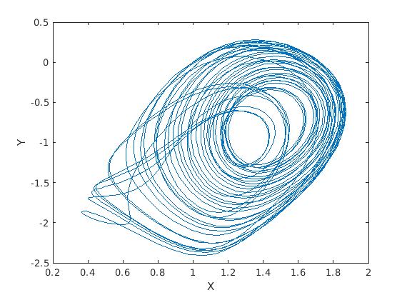
We plot solutions to RF system when α = 1.1 and γ = 0.87 with the initial conditions

\[ x(0) = -1, \quad y(0) = 0, \quad z(0) = 0.5. \]

function rfe
  [t y] = ode45(@rightSide, [0 100], [-1; 0; 0.5]);
  
  plot(-y(:,1), -y(:,2))
  xlabel('X')
  ylabel('Y')
  
%   plot3(y(:,1), y(:,2), y(:,3))
%   xlabel('X')
%   ylabel('Y')
%   zlabel('Z')
  return
  
  function dudt = rightSide(t,y)
    alpha = 1.1;
    gamma = 0.87;
    X = y(1);
    Y = y(2);
    Z = y(3);
    dudt = [Y*(Z - 1 + X^2) + gamma*X; ...
            X*(3*Z + 1 - X^2) + gamma*Y; ...
            -2*Z*(alpha + X*Y)];
%     dudt = [Y.*(Z - 1 + X.^2) + gamma*X; ...
%             X.*(3*Z + 1 - X.^2) + gamma*Y; ...
%             -2*Z.*(alpha + X.*Y)];
        
return

Agrawal, S.K., Srivastava, M., Das, S., Synchronization between fractional-order Ravinovich--Fabrikant and Lotka--Volterra systems, Nonlinear Dynamics, 2014, Vol. 69, No. 4, pp.2277--2288. doi: 10.1007/s11071-012-0426-y
Danca, M.-F., Feckan, M., Kuznetsov, N., Chen, G., Looking more closely to the Rabinovich--Fabrikant system, International Journal of Bifurcation and Chaos, 2016, Vol. 26, No. 2, 1650038 (21 pages).
Danca, M.F., Kuznetsov, N., Chen, G., Unusual dynamics and hidden attractors of the Rabinovich--Fabrikant system, 2016, arXiv:1511.07765
N.V. Kuznetsov, Hidden attractors in fundamental problems and engineering models.A short survey, AETA 2015: Recent Advances in Electrical Engineering and Related Sciences, Lecture Notes in Electrical Engineering, 371 (2016) 13
Rabinovich, M.I. and Fabrikant, A.L., Stochastic self-modulation of waves in nonequilibrium media, J.E.T.P. (Sov.) 77 (1979) 617.

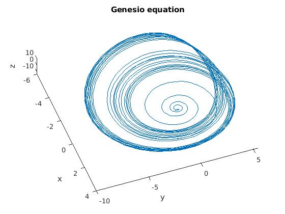
The Genesio equation is

\begin{equation} \label{EqChaos.2} \dddot{x} + a\,\ddot{x} + b\,\dot{x} + c\,x - x^2 =0 , \end{equation}

where 𝑎, b, and c are some constants. Numerical experiments show that system \eqref{EqChaos.2} exhibits a chaotic behavior when

\[ x(0) = 0.2, \quad y(0) = -0.3, \quad z(0) = 1; \qquad a=1.2, \quad b = 2.92, \quad c=6. \]


clear all
genesio();
function genesio()
    
    % initial conditions
    x0 = 0.2;
    y0 = -0.3;
    z0 = 1;
    % numerically solve 
    [t y] = ode45(@genesio_ode, [0 100], [x0; y0; z0]);
    
    % plot
    figure
    plot3(y(:,1),y(:,2),y(:,3));
    xlabel('x');
    ylabel('y');
    zlabel('z');
    title('Genesio equation')

    function dudt = genesio_ode(t,y)
        % parameters
        a = 1.2;
        b = 2.92;
        c = 6;
        
        dudt = [y(2);
                y(3);
                -a*y(3)-b*y(2)-c*y(1)-y(1)^2];
    end
end

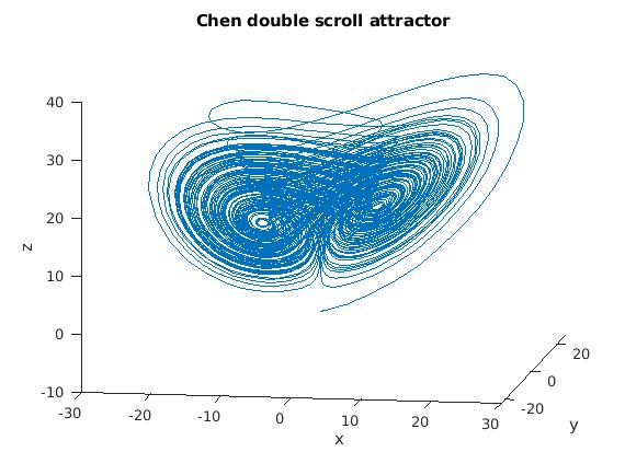
The Chen double scroll attractor is a system of ODEs is models morphogenesis in higher organisms.

\begin{equation} \label{EqChaos.4} \begin{split} \frac{{\text d} x}{{\text d}t} &= a \left( y-x \right) , \\ \frac{{\text d} y}{{\text d}t} &= \left( c - a \right) x - xz + c\,y , \\ \frac{{\text d} z}{{\text d}t} &= xy-b\,z, \end{split} \end{equation}

with \[ a = 40, \quad b =3, \quad c = 28 \qquad\mbox{and initial conditions} \qquad x_0 = -0.1, \quad y_0 = 0.5, \quad z_0 = -0.6 . \]


clear all
chen();
function chen()

    % initial conditions
    x0 = -0.1;
    y0 = 0.5;
    z0 = -0.6;
    % numerically solve 
    [t y] = ode45(@chen_ode, [0 1e2], [x0; y0; z0]);
    
    % plot
    figure
    plot3(y(:,1),y(:,2),y(:,3));
    xlabel('x');
    ylabel('y');
    zlabel('z');
    title('Chen double scroll attractor')  
    
    function dudt = chen_ode(t,y)
        % parameters
        a = 40;
        b = 3;
        c = 28;
        
        dudt = [a*(y(2)-y(1));
                (c-a)*y(1) - y(1)*y(3) + c*y(2);
                y(1)*y(2) - b*y(3)];
    end
end

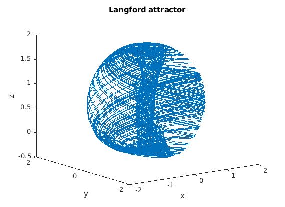
The Langford attractor appear in three dimensional (3D) systems of ODEs.

\begin{equation} \label{EqChaos.5} \begin{split} \dot{x} &= \left( z - b \right) x - d\,y , \\ \dot{y} &= d\,x + \left( z-b \right) y , \\ \dot{z} &= c + a\,z - z^3 /3 - \left( x^2 + y^2 \right) \left( 1 + e\,z \right) + 0.1\,zx^3 . \end{split} \end{equation}

We use the following numerical values

\[ a=0.95, \quad b = 0.7, \quad c = 0.6, \quad d=3.5, \quad e= 0.25, \]

and initial conditions:

\[ x_0 = 0.1, \quad y_0 =1, \quad z_0 = 0. \]


clear all
langford();
%% Langford attractor

function langford()

    % initial conditions
    x0 = 0.1;
    y0 = 1;
    z0 = 0;
    % numerically solve 
    [t y] = ode45(@langford_ode, [0 5e2], [x0; y0; z0]);
    
    % plot
    figure
    plot3(y(:,1),y(:,2),y(:,3));
    xlabel('x');
    ylabel('y');
    zlabel('z');
    title('Langford attractor')  
    
    function dudt = langford_ode(t,y)
        % parameters
        a = 0.95;
        b = 0.7;
        c = 0.6;
        d = 3.5;
        e = 0.25;
        
        dudt = [(y(3) - b)*y(1) - d*y(2);
                d*y(1) + (y(3)-b)*y(2);
                c + a*y(3)-(y(3)^3)/3 - (y(1)^2+y(2)^2)*(1+e*y(3)) + 0.1*y(3)*y(1)^3];
    end
end

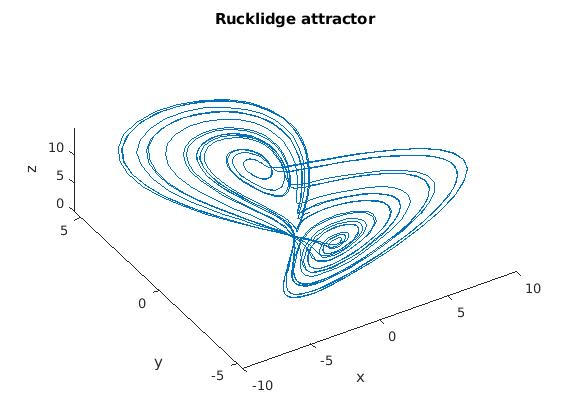
The Rucklidge attractor appear in three dimensional (3D) systems of ODEs.

\begin{equation} \label{EqChaos.7} \begin{split} \dot{x} &= \kappa\, x - \lambda\,y -yz , \\ \dot{y} &= x, \\ \dot{z} &= -z + y^2 . \end{split} \end{equation}

We use the following numerical values

\[ \kappa = -2, \quad \lambda = -6.7 \]

and initial conditions:

\[ x_0 = 1, \quad y_0 = 0, \quad z_0 = 4.5 . \]


clear all
rucklidge();
%% Rucklidge attractor

function rucklidge()

    % initial conditions
    x0 = 1;
    y0 = 0;
    z0 = 4.5;
    % numerically solve 
    [t y] = ode45(@rucklidge_ode, [0 150], [x0; y0; z0]);
    
    % plot
    figure
    plot3(y(:,1),y(:,2),y(:,3));
    xlabel('x');
    ylabel('y');
    zlabel('z');
    title('Rucklidge attractor')  
    function dudt = rucklidge_ode(t,y)
        % parameters
        k = -2;
        l = -6.7;
        
        dudt = [k*y(1) - l*y(2) - y(2)*y(3);
                y(1);
                -y(3) + y(2)^2];
    end
end

Rucklidge attractor. Mathematica code

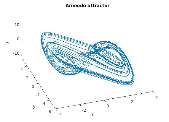
The Arneodo attractor is

\begin{equation} \label{EqChaos.8} \dddot{x} + \ddot{x} + b\,\dot{x} + a\,x +c\, x^3 =0 , \end{equation}

where 𝑎, b, and c are some constants. Numerical experiments show that system \eqref{EqChaos.8} exhibits a chaotic behavior when

\[ x(0) = 0.2, \quad y(0) = 0.2, \quad z(0) = -0.75; \qquad a=-5.5, \quad b = 3.5, \quad c=1. \]


clear all
arneodo();%% Arneodo attractor

function arneodo()
    
    % initial conditions
    x0 = 0.2;
    y0 = 0.2;
    z0 = -0.75;
    % numerically solve 
    [t y] = ode45(@arneodo_ode, [0 200], [x0; y0; z0]);
    
    % plot
    figure
    plot3(y(:,1),y(:,2),y(:,3));
    xlabel('x');
    ylabel('y');
    zlabel('z');
    title('Arneodo attractor')

    function dudt = arneodo_ode(t,y)
        % parameters
        a = -5.5;
        b = 3.5;
        c = 1;
        
        dudt = [y(2);
                y(3);
                -y(3)-b*y(2)-a*y(1)-c*y(1)^3];
    end
end

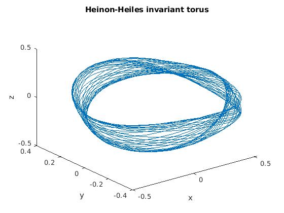
The Hénon-Heiles invariant torus models the motion of individual stars as affected by the rest of a galaxy. Unlike the other models, this is a four-dimensional example. We project and only plot(𝑥,𝑦,𝑧). The system is Hamiltonian, so the chaotic solutions are not strange attractor.

\begin{equation} \label{EqChaos.9} \begin{split} \dot{x} &= z , \\ \dot{y} &= w, \\ \dot{z} &= -x-2xy , \\ \dot{w} &= -y-x^2 + y^2 . \end{split} \end{equation}

Initial conditions:

\[ x_0 = 0, \quad y_0 = 0, \quad z_0 = 0.35, \quad w_0 = -0.3 . \]


clear all
henon_heiles();

%% Henon-Heiles invariant torus

function henon_heiles()
    % initial conditions
    x0 = 0;
    y0 = 0;
    z0 = 0.35;
    w0 = -0.3;
    % numerically solve 
    [t y] = ode45(@henon_heiles_ode, [0 200], [x0; y0; z0; w0]);
    
    % plot
    figure
    plot3(y(:,1),y(:,2),y(:,3));
    xlabel('x');
    ylabel('y');
    zlabel('z');
    title('Heinon-Heiles invariant torus')

    function dudt = henon_heiles_ode(t,y)
        
        dudt = [y(3);
                y(4);
                -y(1) - 2*y(1)*y(2);
                -y(2)-y(1)^2 + y(2)^2];
    end
end

Examples of Chaotic Equations

Poincaré Map