--->
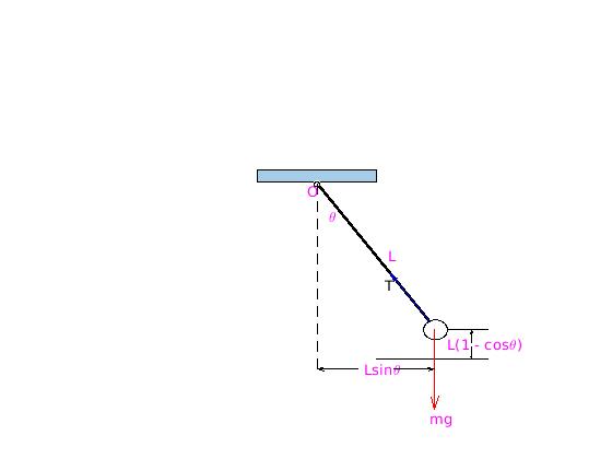
A simple pendulum consists of a single point of mass
m (bob) attached
to a rod (or wire) of length
\( \ell \) and of
negligible weight. We denote by θ the angle measured between the
rod and the vertical axis, which is assumed to be positive in
counterclockwise direction.
We consider the simple pendulum that is characterized by the following assumptions:
-
The bob is free to move within a plane (so we consider only two-dimensional oscillations).
-
The system is conservative, so the pendulum rotates in a vacuum and friction in the pivot is
negligible.
-
The bob of mass m is attached to one end of a rigid, but weightless rod of length
ℓ, which is assumed to be constant during the pendulum motion. The other end of the rod
(or rigid spring) is supported at the pivot.
|
|
First, we illustrate with matlab the motion
of the simple pendulum. Introducing the function f for circle arrow
top=polyshape([-1 1 1 -1],[0 0 1/4 1/4]);
plot(top);
circle1=viscircles([0 -1/20],1/20,'color','black','linewidth',1);
circle2=viscircles([2 -3],1/5,'color','black','linewidth',1);
line1=line([0, 0], [-1/20, -3.8],'LineStyle','--','color','black');
line2=line([0.03, 1.9], [-0.07, -2.83],'linewidth',2,'color','black');
text1=text(0.8, -3.8,'Lsin\theta','color','magenta','FontName','Times New Roman');
text2=text(1.9, -4.8,'mg','color','magenta','FontName','Times New Roman');
line3=line([1.0, 2.9], [-3.6, -3.6],'color','black');
line4=line([2.2, 2.9], [-3.0, -3.0],'color','black');
text3=text(2.2, -3.3, 'L(1 - cos\theta)','color','magenta','FontName','Times New Roman');
text4 =text(1.2,-1.5,'L','color','magenta','FontName','Times New Roman');
text5 = text(0.2,-0.7,'\theta','color','magenta','FontName','Times New Roman');
text6 = text(-0.16,-0.2,'O','color','magenta','FontName','Times New Roman');
textT = text(1.15,-2.1,'T','color','black','FontName','Times New Roman');

%arrow
hold on
p1 = [1.986, -3.0];                         % First Point
p2 = [1.986, -4.6];                         % Second Point
dp = p2-p1;                         % Difference
figure(1)
quiver(p1(1),p1(2),dp(1),dp(2),0,'color','r','MaxHeadSize',0.5)

%arrow2a
hold on
p1 = [0.7, -3.8];                         % First Point
p2 = [0, -3.8];                         % Second Point
dp = p2-p1;                         % Difference
figure(1)
quiver(p1(1),p1(2),dp(1),dp(2),0,'color','black','MaxHeadSize',0.5)
%arrow2b
hold on
p1 = [1.3, -3.8];                         % First Point
p2 = [1.98, -3.8];                         % Second Point
dp = p2-p1;                         % Difference
figure(1)
quiver(p1(1),p1(2),dp(1),dp(2),0,'color','black','MaxHeadSize',0.5)
%arrow3a
hold on
p1 = [2.6, -3.35];                         % First Point
p2 = [2.6, -3.6];                         % Second Point
dp = p2-p1;                         % Difference
figure(1)
quiver(p1(1),p1(2),dp(1),dp(2),0,'color','black','MaxHeadSize',0.8)
%arrow3b
hold on
p1 = [2.6, -3.27];                         % First Point
p2 = [2.6, -3.0];                         % Second Point
dp = p2-p1;                         % Difference
figure(1)
quiver(p1(1),p1(2),dp(1),dp(2),0,'color','black','MaxHeadSize',0.8)

%arrowT
hold on
p1 = [1.9 -2.83];                         % First Point
p2 = [1.25 -1.86184];                         % Second Point
dp = p2-p1;                         % Difference
figure(1)
quiver(p1(1),p1(2),dp(1),dp(2),0,'color','b','MaxHeadSize',0.5)

hold on

axis off
xlim([-4 4]);
ylim([-4 3]);

%arc
P = plot_arc(-pi/2,-0.98,0,0,1);
set(P,'color','black','linewidth',1,'LineStyle','--')

%arctheta
P = plot_arc(-pi/2,-0.98,0,0,3.6);
set(P,'color','black','linewidth',1,'LineStyle','--')

function P = plot_arc(a,b,h,k,r)
% Plot a circular arc as a pie wedge.
% a is start of arc in radians,
% b is end of arc in radians,
% (h,k) is the center of the circle.
% r is the radius.
% Try this:   plot_arc(pi/4,3*pi/4,9,-4,3)
% Author:  Matt Fig
t = linspace(a,b);
x = r*cos(t) + h;
y = r*sin(t) + k;
x = [x h x(1)];
y = [y k y(1)];
P = plot(x,y);
% axis([h-r-1 h+r+1 k-r-1 k+r+1])
% axis square;
if ~nargout
    clear P
end
end
|
|
Figure 1: Simple pendulum.
|
|
matlab code
|

|
|
The modeling of the motion is greatly simplified when the given body (bob) is considered
essentially as a point particle. The position of the bob is described by the angle θ
between the rod and the downward equilibrium vertical position, with the counterclockwise
direction taken as positive. The only force acting on the pendulum is the gravitational
force m g, acting downward, where g denotes the acceleration
due to gravity. The position of the bob can be determined in Cartesian
coordinates as
\[
x = \ell \,\sin \theta , \qquad y = -\ell\,\cos\theta ,
\]
where the origin is taken at the pivot and the positive vertical direction is upward.
Using \( {\cal L} = \mbox{K} - \Pi , \) the
Lagrangian,
which is the difference of the kinetic energy K and the potential
energy Π of the system, we have
\[
\frac{\text d}{{\text d}t} \,\frac{\partial {\cal L}}{\partial \dot{\theta}}
= \frac{\partial {\cal L}}{\partial \theta} .
\]
|
With the kinetic energy expressed via the angular displacement θ
\[
\mbox{K} = \frac{m}{2} \left( \dot{x}^2 + \dot{y}^2 \right) = \frac{m}{2}\, \ell^2 \left[
\left( \dot{\theta} \,\cos\theta \right)^2 + \left( \dot{\theta} \,\sin \theta \right)^2
\right] = \frac{m}{2}\,\ell^2 \dot{\theta}^2 .
\]
and the potential energy
\[
\Pi = mg \left( \ell + y \right) = mg\ell \left( 1- \cos \theta \right) ,
\]
we derive the corresponding derivatives
\[
\frac{\partial \mbox{K}}{\partial \dot{\theta}} = I_0 \dot{\theta} = m\ell^2 \dot{\theta} ,
\qquad
\frac{\partial \Pi}{\partial \theta} = mgy = mg\ell \, \sin \theta .
\]
Using these expressions, we obtain from the Euler--Lagrange equation
\( \displaystyle \frac{\text d}{{\text d} t} \left( \frac{\partial {\cal
L}}{\partial \dot{\theta}} \right) =
\frac{\partial {\cal L}}{\partial \theta} , \) for the Lagrangian
\( {\cal L} = \mbox{K} - \Pi , \) the pendulum equation in a vacuum:
\[
\ddot{\theta} + \left( g/\ell \right) \sin \theta =0 \qquad \mbox{or} \qquad \ddot{\theta} +
\omega_0^2 \sin \theta =0 \qquad \left( \omega_0^2 =
g/\ell \right) ,
\]
where
\( \ddot{\theta} = {\text d}^2 \theta / {\text d}t^2 \) ,
\( \omega_0 = \sqrt{g/\ell} >0 ,\) and
g is
gravitational acceleration.
Further simplification is available by normalization, which leads to \(
\omega = 1 \) and we get
\[
\ddot{\theta} + \sin \theta =0 .
\]
In practice, it is easier to study an ordinary differential equation as a system of equations
involving only the first derivatives.
\[
\dot{x} = y, \qquad \dot{y} = -\sin x .
\]
The variables
x and
y can be interpreted geometrically. Indeed, the angle
x
= θ corresponds to a point on a circle whereas the velocity
\( y =
\dot{\theta} \) corresponds to a point on a real line. Therefore, the set of all
states (x ,y) can be represented by a cylinder, the product of a circle by a line. More
formally, the phase space of the pendulum is the cylinder
\( S^1 \times
\mathbb{R} , \) its elements are couples (position,velocity).
Thus, at each point
(x ,y) in the phase space, there is an attached vector
\( (\dot{x}, \dot{y} ) = (y, - \sin x) . \) This can be geometrically
represented as a
vector field on the cylindrical phase space.
Example:
The swinging mass m has a kinetic energy of
\( m \ell^2 \left( {\text d}\theta /{\text d}t \right)^2 /2 \)
and a potential
energy of \( mg\ell\left( 1 - \cos \theta \right) ; \) the
potential energy is zero for θ = 0. Let θM denote the maximum
amplitude of the pendulum. Since dθ/dt = 0 at θ = θM,
conservation of energy gives
\[
\frac{1}{2} \,m\ell^2 \left( \frac{{\text d}\theta}{{\text d}t} \right)^2 = mg\ell\,\cos
\theta - mg\ell\,\cos \theta_M .
\]
Solving for the velocity dθ/d
t, we obtain
\[
\frac{{\text d}\theta}{{\text d}t} = \pm \left( \frac{2g}{\ell} \right)^{1/2} \left( \cos
\theta - mg\ell\,\cos \theta_M \right)^{1/2} ,
\]
with the mass
m canceling out. We take
t to be zero, when θ = 0 and
dθ/d
t > 0. An integration from θ = 0 t0 θ
M yields
\begin{equation}
\int_0^{\theta_M} \left( \cos \theta - mg\ell\,\cos \theta_M \right)^{-1/2} {\text d}\theta
= \left( \frac{2g}{\ell} \right)^{1/2} \int_0^t {\text d}t = \left( \frac{2g}{\ell}
\right)^{1/2} t .
\label{pendulum.1}
\end{equation}
This is one-fourth of a cycle, and therefore the time
t is one-fourth of the period,
T. We note that θ < θ
M, and with a bit of clairvoyance we try
the half-angle
substitution
\[
\sin \frac{\theta}{2} = \sin \left( \frac{\theta_M}{2} \right) \sin \phi .
\]
With this, Eq.\eqref{pendulum.1} becomes
\begin{equation}
T = 2\pi \left( \frac{\ell}{g} \right)^{1/2} \int_0^{\pi} \left[ 1 - \sin^2 \left(
\frac{\theta_M}{2} \right) \sin^2 \phi \right]^{-1/2} {\text d}\phi .
\label{pendulum.2}
\end{equation}
Although not an obvious improvement over Eq.\eqref{pendulum.1}, the integral
\eqref{pendulum.2} now defines the complete elliptic integral of the first kind,
\( K \left( \sin^2 \theta_M /2 \right) . \)
From the
series expansion, the period of our pendulum may be developed as a power
series—powers of sin θ
M/2:
\[
T = 2\pi \left( \frac{\ell}{g} \right)^{1/2} \left\{1 + \frac{1}{4}\,\sin^2
\frac{\theta_M}{2} + \frac{9}{64}\,\sin^4 \frac{\theta_M}{2} + \cdots \right\} .
\]
■
We convert the pendulum equation with resistance
\[
m\ell^2 \ddot{\theta} + c\,\dot{\theta} + mg\ell \,\sin \theta =0 .
\]
to a system of two first order equations by letting
\( x= \theta
\quad\mbox{and} \quad y = \dot{\theta} : \)
\[
\frac{{\text d} x}{{\text d}t} = y , \qquad \frac{{\text d} y}{{\text d}t} = -\omega^2 \sin x
- \gamma \,y .
\]
Here
\( \gamma = c/(m\,\ell ) , \ \omega^2 = g/\ell \) are positive
constants. Therefore, the above system of differential equations is autonomous. Setting
\( \gamma = 0.25 \quad\mbox{and}\quad \omega^2 =1 , \) we ask
Mathematica to provide a phase portrait for the pendulum equation with resistance:
Let us consider a rod of length ℓ of mass
m with attached ball of mass
M at a
distance
L from the pivot.

|
|
rod = Graphics[{LightGray,
Polygon[{{0.1, 0}, {0, 0.1}, {2.0, 2.1}, {2.1, 2.0}}]}];
ball = Graphics[{Orange, Disk[{1.75, 1.75}, 0.25]}];
ar3 = Graphics[{Black, Dashed, Thickness[0.01], Arrowheads[0.08],
Arrow[{{1, 1}, {1, 0.4}}]}];
ar = Graphics[{Black, Thickness[0.01], Arrowheads[0.08],
Arrow[{{-0.2, 0}, {2.5, 0}}]}];
ar2 = Graphics[{Black, Dashed, Thickness[0.01], Arrowheads[0.08],
Arrow[{{0, -0.2}, {0, 2.2}}]}];
tl = Graphics[{Black,
Text[Style["\[ScriptL]", 18, FontFamily -> "Mathematica1"], {1.2,
1.45}]}];
tx = Graphics[{Black, Text[Style["x", 18], {2.4, 0.2}]}];
tm = Graphics[{Black,
Text[Style["M", 18, FontFamily -> "Mathematica1"], {1.4, 1.75}]}];
t1 = Graphics[{Black, Text[Style["C", 18], {1.0, 1.2}]}];
t2 = Graphics[{Black, Text[Style["\[Theta]", 18], {0.15, 0.4}]}];
t3 = Graphics[{Black, Text[Style["mg", 18], {1.05, 0.3}]}];
Show[rod, ar, ar2, ar3, tx, tl, tm, t1, t2, t3, ball]
|
|
Rigid pendulum with a ball.
|
|
Mathematica code
|
To analyze the problem of falling meterstick of length ℓ with attached heavy weight at a
distance
L from the pivot, we use the tourque equation:
\[
I\,\ddot{\theta} = \tau
\]
is the torque. This yields
\[
I\,\ddot{\theta} = \left( \frac{m}{2}\,g\,\ell + Mg\,L \right) \sin\theta ,
\]
where θ = θ(
t) is the instanteneous angle of the rod with the vertical axis,
and
\( \displaystyle I = \frac{m}{3}\,\ell^2 + M\,L^2 \) is the
moment of inertia about the lower
end.
Introducing the dimensionless ratios
k =
M/
m and
q =
L/ℓ,
we can express the angular acceleration of the loaded stick in terms of the angular acceleration
of the bare meterstick and a dimensionless factor:
\[
\ddot{\theta} = \frac{3g}{2\ell}\cdot \frac{1 + 2kq}{1 + kq^2} \cdot \sin\theta .
\]
It is instructive to examine the dimensionless factor in the previous equation of motion. For
q = ⅔, it equals 1 for all values of
k. Adding any point mass at ⅔
of the length ℓ of a uniform rod leaves the angular acceleration and, therefore, the time of
fall unchanged. For
q < ⅔, the factor becomes greater than 1, and the time of
fall gets shorter. The opposite is true for
q > ⅔.
k*
Consider the motion under gravity of a bob of mass
m attached to a fixed point by an
inextensible massless rod of length ℓ. The bob is free to move on a sphere of radius ℓ.
Using spherical coordinates (angles) θ and ϕ as the generalized coordinates,
the kinetic and potential energies become
\begin{align*}
\mbox{K} &= \frac{m}{2}\,\ell^2 \left( \dot{\theta}^2 + \dot{\phi}^2 \sin^2 \theta \right) ,
\\
\Pi &= mg\ell \left( 1- \cos \theta \right) .
\end{align*}
This allows us to derive the Euler--Lagrange equations for the corresponding Lagrangian:
\[
\frac{\text d}{{\text d}t} \left( \frac{\partial {\cal L}}{\partial \dot{\theta}} \right) -
\frac{\partial {\cal L}}{\partial \theta} = 0 , \qquad
\frac{\text d}{{\text d}t} \left( \frac{\partial {\cal L}}{\partial \dot{\phi}} \right) -
\frac{\partial {\cal L}}{\partial \phi} = 0 .
\]
Substituting the expressions for the kinetic and potential energies, we obtain
two coupled equations
\[
\begin{split}
\ddot{\theta} + \frac{g}{\ell} \,\sin\theta - \frac{1}{2} \,\dot{\phi}^2 \sin 2\theta &= 0,
\\
\ddot{\phi}\,\sin\theta + 2\dot{\phi} \dot{\theta}\,\cos\theta &= 0.
\end{split}
\]
The last equation is a first order differential equation with respect to the derivative of
ϕ, so it can be integrated
\[
\dot{\phi} \sin^2 \theta = c, \quad \mbox{a constant}.
\]
Using this equation, we obtain the following differential equation for nagle θ:
\[
\dot{\theta} + \frac{g}{\ell} \,\sin\theta - \frac{c^2 \cos\theta}{\sin^3 \theta} = 0.
\]
The length of the pendulum is increasing by stretching of the wire due to the weight of the
bob. The effective
spring constant for a wire of rest length \( \ell_0 \) is
\[
k = ES/ \ell_0 ,
\]
where the elastic modulus (Young's modulus) for steel is about
\( E \approx
2.0 \times 10^{11} \)
Pa and
S is the cross-sectional area. With pendulum 3 m long, the static increase in
elongation is about
\( \Delta \ell = 1.6 \) mm, which is clearly not negligible. There
is also dynamic
stretching of the wire from the apparent centrifugal and Coriolis forces acting on the bob
during motion. We can
evaluate this effect by adapting a spring-pendulum system analysis. WE go from rectangular to
polar coordinates:
\[
x= \ell \,\sin \theta = z_0 \left( 1 + \xi \right) \sin \theta , \qquad z= z_0 - \ell\,\cos
\theta = z_0 \left[ 1 - \left( 1 + \xi \right) \cos \theta \right] , ,
\]
where
\( z_0 = \ell_0 + mg/k \) is the static pendulum length,
\( \ell = z_0 \left( 1 + \xi \right) \) is the dynamic length, ξ
is the fractional
string extension, and θ is the deflection angle. the equations of motion for small
deflections are
\begin{eqnarray*}
\left( 1 + \xi \right)\ddot{\theta} + 2\dot{\theta}\,\dot{\xi} + \omega_p^2 \theta &=& 0 , \\
\ddot{\xi} + \omega_s^2 \xi - \dot{\theta} + \frac{1}[2}\,\omega_p^2 \theta^2 &=& 0,
\end{equarray*}
where the overdots denote differentiation with respect to time
t,
\(
\omega_p^2 = g/z_0 \)
is the square of the pendulum frequency, and
\( \omega_s^2 = k/m \)
is the spring
(string) frequency, squared.
To get a feeling for how rigid and massive the pendulum support must be, we model the support
as mass M
kept in place by a spring of constant K, as shown in the picture below.
p = Rectangle[{-Pi/6 - 1.2, 2}, {-5, -5}]
a = Graphics[{Gray, p}]
coil = ParametricPlot[{t + 1.2*Sin[3*t],
1.2*Cos[3*t] - 1.2}, {t, -Pi/6 , 5*Pi - Pi/6}, FrameTicks -> None,
PlotStyle -> Black]
line = Graphics[{Thick, Line[{{16.3843645, -1.2}, {20, -1.2}}]}]
r = Graphics[{EdgeForm[{Thick, Blue}], FaceForm[],
Rectangle[{20, -5}, {26, 2}]}]
back = RegionPlot[-5 < x < 28 || -7 < y < -5, {x, -5, 28}, {y, -7, -5}, PlotStyle ->
LightOrange]
line2 = Graphics[{Thick, Dashed, Line[{{23, -1}, {23, -14}}]}]
line3 = Graphics[{Thick, Line[{{23, -1}, {29, -11.5}}]}]
disk = Graphics[{Pink, Disk[{29.5, -12}, 1]}]
text = Graphics[Text["\[Theta]" , {25.1, -9.5}]]
Show[a, coil, line, r, back, line2, line3, disk, text]
Pendulum with moving support.
The natural frequency of the support is
\[
\Omega = \left( K/M \right)^{1/2} .
\]
The coupled equations for the system are
\begin{eqnarray*}
\ddot{\theta} + \omega_0^2 \theta + \ddot{x}/\ell &=& 0 , \\
\left( 1 + m/M \right) \ddot{x} + \left( m/M \right) \ell \,\ddot{\theta} + \Omega^2 x &=&
0,
\end{eqnarray*}
where
x is the displacement of the rigid support. The former equation says that the
effect of sway is to
impart an additional angular acceleration
\( - \ddot{x}/\ell \) to
the pendulum
for small angles of oscillation (otherwise, we have to use
\( \omega_0^2
\sin \theta \)
instead of
\( \omega_0^2 \theta \) ).
function main
tstart=0;
tstop=20;
z0=0; z0prime=1; theta0=0.1; theta0prime=0.1;
initial_w=[z0, theta0,z0prime,theta0prime]
k=50 ; m=2;  g=9.81;
l=0.5+m*g/k;
[times,sols]=ode45(@(t,w) diffeq(t,w,k,m,l,g), [tstart,tstop],initial_w)

figure
comet(sols(:,1),sols(:,2))
title('Theta vs z')
xlabel('z'),ylabel('theta (rad)')

figure
comet((times),sols(:,1))
title('z vs time')
xlabel('time'),ylabel('z')

figure
comet((times),sols(:,2))
title('Theta vs time')
xlabel('time'),ylabel('theta (rad)')

end
function dwdt=diffeq(t,w,k,m,l,g)
u1=w(1); u2=w(3); v1=w(2); v2=w(4);
du1dt=u2;
du2dt=-k/m*u1-g/(2*l)*v1^2+v2^2;
dv1dt=v2;
dv2dt=1/(1+2*u1)*(-g/l*v1-g/l*u1*v1-2*u2*v2);
dwdt=[du1dt;dv1dt;du2dt;dv2dt];
function spring

%Initial Conditions
initial_w=[0;0.1;1.5;0.1];
m=.2; k=5; g=9.8; l=.5+(m*g/k);

%Solves differential equation
[time,sols]=ode45(@(t,w) diffeq(t,w,m,k,g,l),[0,20],initial_w) %column 1 of solutions is z(t), column 2 is theta(t), column 3 is z'(t), column 4 is theta'(t)
%Plots path
figure
comet(sols(:,1),sols(:,2)) %Plots z vs theta
title('Displacement vs Theta')
xlabel('Theta (rad)')
ylabel('Displacement')

figure
comet(time,sols(:,1)) %Plots z vs time
title('Displacement vs Time')
xlabel('Time (s)')
ylabel('Displacement')

figure
comet(time,sols(:,2)) %Plots theta vs time
title('Theta vs Time')
xlabel('Time (s)')
ylabel('Theta (rad)')

end
function dwdt = diffeq(t,w,m,k,g,l)
z=w(1); theta=w(2); vz=w(3); vtheta=w(4) %Assigns values from vector w
dzdt=vz; dthetadt=vtheta;

dvzdt=-((k/m)*z + (g/(2*l))*theta^2 - vtheta^2)
dvthetadt= -((g/l)*theta + (g/(2*l))*z*theta + 2*vz*vtheta)/(1+2*z)

dwdt=[dzdt;dthetadt;dvzdt;dvthetadt]; %Puts derivatives into matrix dwdt

end
|
Double pendulum.
|
Double compound pendulum.
|
Animation of double pendulum.
|
A double pendulum consists of one pendulum attached to another. Double pendula are an
example of a simple physical
system which can exhibit chaotic behavior with a strong sensitivity to
initial conditions. Several variants of the double pendulum may be considered; the two limbs
may be of equal or unequal lengths and masses, they may be simple pendulums/pendula or
compound pendulums (also called complex pendulums) and the motion may be in three dimensions
or restricted to the vertical plane.
Consider a double bob pendulum with masses m1 and
m2 attached by rigid massless wires of lengths \(
\ell_1 \) and
\( \ell_2 . \)
Further, let the angles the two wires make with the vertical be denoted
\( \theta_1 \) and
\( \theta_2 , \) as illustrated at the
left.
Let the origin of the Cartesian coordinate system is taken to be at
the point of suspension of the first pendulum, with vertical axis
pointed up.
Finally, let gravity be given by g.
Then the positions of the bobs are given by
\begin{eqnarray*}
x_1 &=& \ell_1 \sin \theta_1 , \\
y_1 &=& -\ell_1 \cos \theta_1 , \\
x_2 &=& \ell_1 \sin \theta_1 + \ell_2 \sin \theta_2 , \\
y_2 &=& -\ell_1 \cos \theta_1 - \ell_2 \cos \theta_2 .
\end{eqnarray*}
The potential energy of the system is then given by
\[
\Pi = g\, m_1 \left( \ell_1 + y_1 \right) + g\,m_2 \left( \ell_1 +
\ell_2 + y_2 \right) = g\,m_1 \left( 1- \cos \theta_1 \right) + g\,
m_2 \left( \ell_1 + \ell_2 - \ell_1 \cos \theta_1 - \ell_2 \cos \theta_2 \right) ,
\]
and the kinetic energy by
\begin{eqnarray*}
\mbox{K} &=& \frac{1}{2}\, m_1 v_1^2 + \frac{1}{2}\, m_2 v_2^2 \\
&=& \frac{1}{2}\, m_1 \ell_1^2 \dot{\theta}_1^2 + \frac{1}{2}\, m_2 \left[ \ell_1^2
\dot{\theta}_1^2 +
\ell_2^2 \dot{\theta}_2^2 +2\ell_1 \ell_2 \dot{\theta}_1 \dot{\theta}_2 \cos \left( \theta_1
- \theta_2 \right) \right]
\end{eqnarray*}
because
\[
v_1^2 = \dot{x}_1^2 + \dot{y}_1^2 = \ell_1^2 \dot{\theta}_1^2 , \qquad
v_2^2 = \dot{x}_2^2 + \dot{y}_2^2 = \left( \ell_1 \cos\theta_1
\,\dot{\theta}_1 + \ell_2 \cos \theta_2 \,\dot{\theta}_2 \right)^2 + \left( \ell_1
\sin\theta_1
\,\dot{\theta}_1 + \ell_2 \sin \theta_2 \,\dot{\theta}_2 \right)^2 .
\]
The Lagrangian is then
\begin{eqnarray*}
{\cal L} &=& \mbox{K} - \Pi \\
&=& \frac{1}{2}\, m_1 \ell_1^2 \dot{\theta}_1^2 + \frac{1}{2}\, m_2 \left[ \ell_1^2
\dot{\theta}_1^2 +
\ell_2^2 \dot{\theta}_2^2 +2\ell_1 \ell_2 \dot{\theta}_1 \dot{\theta}_2 \cos \left( \theta_1
- \theta_2 \right) \right]
+ \left( m_1 + m_2 \right) g\ell_1 \cos \theta_1 + m_2 g \ell_2 \cos \theta_2 .
\end{eqnarray*}
Therefore, for θ
1 we have
\begin{eqnarray*}
\frac{\partial {\cal L}}{\partial \dot{\theta}_1} &=& m_1 \ell_1^2 \dot{\theta}_1 + m_2
\ell_1^2 \dot{\theta}_1 +
m_2 \ell_1 \ell_2 \dot{\theta}_2 \cos \left( \theta_1 - \theta_2 \right) , \\
\frac{{\text d}}{{\text d}t} \left( \frac{\partial {\cal L}}{\partial \dot{\theta}_1}
\right) &=&
\left( m_1 + m_2 \right) \ell_1^2 \ddot{\theta}_1 + m_2 \ell_1 \ell_2 \ddot{\theta}_2 \cos
\left( \theta_1 - \theta_2 \right) -
m_2 \ell_1 \ell_2 \dot{\theta}_2 \sin \left( \theta_1 - \theta_2 \right) \left(
\dot{\theta}_1 - \dot{\theta}_2 \right) ,
\\
\frac{\partial {\cal L}}{\partial \theta_1} &=& - \ell_1 g \left( m_1 + m_2 \right) \sin
\theta_1 - m_2 \ell_1 \ell_2 \dot{\theta}_1 \dot{\theta}_2 \sin \left( \theta_1 - \theta_2
\right) .
\end{eqnarray*}
So the Euler-Lagrange differential equation
\( \frac{{\text d}}{{\text d}t}
\left( \frac{\partial {\cal L}}{\partial \dot{q}} \right) = \frac{\partial {\cal
L}}{\partial q} \)
for θ
1 becomes
\[
\left( m_1 + m_2 \right) \ell_1^2 \ddot{\theta}_1 + m_2 \ell_1 \ell_2 \ddot{\theta}_2 \cos
\left( \theta_1 - \theta_2 \right)
+ m_2 \ell_1 \ell_2 \dot{\theta}_2^2 \sin \left( \theta_1 - \theta_2 \right) + \ell_1 g
\left( m_1 + m_2 \right) \sin \theta_1 =0 .
\]
Dividing through by
\( \ell_1 , \) this simplifies to
\[
\left( m_1 + m_2 \right) \ell_1 \ddot{\theta}_1 + m_2 \ell_2 \ddot{\theta}_2 \cos \left(
\theta_1 - \theta_2 \right)
+ m_2 \ell_2 \dot{\theta}_2^2 \sin \left( \theta_1 - \theta_2 \right) + g \left( m_1 + m_2
\right) \sin \theta_1 =0 .
\]
Similarly, for θ
2, we have
\begin{eqnarray*}
\frac{\partial {\cal L}}{\partial \dot{\theta}_2} &=& m_2 \ell_2^2 \dot{\theta}_2 + m_2
\ell_1 \ell_2 \dot{\theta}_1
\cos \left( \theta_1 - \theta_2 \right) , \\
\frac{{\text d}}{{\text d}t} \left( \frac{\partial {\cal L}}{\partial \dot{\theta}_2}
\right) &=&
m_2 \ell_2^2 \ddot{\theta}_2 + m_2 \ell_1 \ell_2 \ddot{\theta}_1 \cos \left( \theta_1 -
\theta_2 \right) -
m_2 \ell_1 \ell_2 \dot{\theta}_1 \sin \left( \theta_1 - \theta_2 \right) \left(
\dot{\theta}_1 - \dot{\theta}_2 \right) ,
\\
\frac{\partial {\cal L}}{\partial \theta_2} &=& \ell_1 \ell_2 m_2 \dot{\theta}_1
\dot{\theta}_2
\sin \left( \theta_1 - \theta_2 \right) - \ell_2 m_2 g\,\sin \theta_2 ,
\end{eqnarray*}
which leads to
\[
m_2 \ell_2 \ddot{\theta}_2 + m_2 \ell_1 \ddot{\theta}_1 \cos \left( \theta_1 - \theta_2
\right)
- m_2 \ell_1 \dot{\theta}_1^2 \sin \left( \theta_1 - \theta_2 \right) + m_2 g \, \sin
\theta_2 =0 .
\]
The coupled second-order ordinary differential equations
\begin{eqnarray*}
\left( m_1 + m_2 \right) \ell_1 \ddot{\theta}_1 + m_2 \ell_2 \ddot{\theta}_2 \cos \left(
\theta_1 - \theta_2 \right)
+ m_2 \ell_2 \dot{\theta}_2^2 \sin \left( \theta_1 - \theta_2 \right) + g \left( m_1 + m_2
\right) \sin \theta_1 &=& 0 ,
\\
m_2 \ell_2 \ddot{\theta}_2 + m_2 \ell_1 \ddot{\theta}_1 \cos \left( \theta_1 - \theta_2
\right)
- m_2 \ell_1 \dot{\theta}_1^2 \sin \left( \theta_1 - \theta_2 \right) + m_2 g \, \sin
\theta_2 &=& 0
\end{eqnarray*}
The equations of motion can also be written in the Hamiltonian formalism. Computing the
generalized momenta gives
\begin{eqnarray*}
p_1 &=& \frac{\partial {\cal L}}{\partial \dot{\theta}_1} = \left( m_1 + m_2 \right)
\ell_1^2 \dot{\theta}_1 + m_2 \ell_1 \ell_2 \dot{\theta}_2
\cos \left( \theta_1 - \theta_2 \right) ,
\\
p_2 &=& \frac{\partial {\cal L}}{\partial \dot{\theta}_2} = m_2 \ell_2^2 \dot{\theta}_2 +
m_2 \ell_1 \ell_2 \dot{\theta}_1
\cos \left( \theta_1 - \theta_2 \right) .
\end{eqnarray*}
The Hamiltonian becomes
\[
H = \dot{\theta}_1 p_1 + \dot{\theta}_2 p_2 - {\cal L} .
\]
For animationof double pendulum equations, see:
https://www.myphysicslab.com/pendulum/double-pendulum-en.html
function DoublePendulum
  [l1,l2,~,~,~,s]=pendata;  % parameters
  ax1=[-s s -s s]; % vector for axes
  T = 25; % Process duration, s
  v = 3;  % Speed of animation, positive integer: 1, 2, 3,...
% Initial values
  theta1_1 = pi/2;
  theta1 = 0;
  theta2_1 = pi/2;
  theta2 = 0;
  y0 = [theta1_1, theta1, theta2_1, theta2];

  [t,y] = ode45(@Equations, [0, T], y0);
  x1 = l1*sin(y(:,1));
  y1 = -l1*cos(y(:,1));
  x2 = x1 + l2*sin(y(:,3));
  y2 = y1 - l2*cos(y(:,3));

  figure
  tic
%   Animation
  for i = 1:v:numel(t)
   plot(0, 0,'k.',x1(i),y1(i),'b.',x2(i),y2(i),'r.','markersize',40);
   axis(ax1)
   line([0 x1(i)], [0 y1(i)],'Linewidth',2);
   line([x1(i) x2(i)], [y1(i) y2(i)],'linewidth',2,'color','r');
   xlabel(['\it\bf X \rm        Animation time, s:  ',num2str(toc,3)],...
     'HorizontalAlignment', 'left');
   ylabel('\it\bf Y');
   title(['Double Pendulum       \it t \rm= ',num2str(t(i),3)],...
     'fontsize',13, 'HorizontalAlignment', 'left', 'Position',[-.4*s s 0])
   drawnow
  end

%   Graphs
  figure
  plot(x1,y1,x2,y2,'r')
  xlabel('\it X','fontSize',12);
  ylabel('\it Y','fontSize',12);
  title('Chaotic Motion of a Double Pendulum')

  figure
  plot(t,y(:,1),t,y(:,3),'r','linewidth',2)
  axis([0,T,min(y(:,3)),max(y(:,3))])
  legend('\theta_1','\theta_2')
  xlabel('Time, s','fontSize',12)
  ylabel('\theta','fontSize',18,'fontweight','bold')
  title('\theta_1(0) = \pi/2  and  \theta_2(0) = \pi/2','fontsize',13)
 end

function z = Equations(~, y)
  [l1,l2,m1,m2,g,~]=pendata;
  z(4,1)=0;
  a = (m1+m2)*l1 ;
  b = m2*l2*cos(y(1)-y(3)) ;
  c = m2*l1*cos(y(1)-y(3)) ;
  d = m2*l2 ;
  e = -m2*l2*y(4)* y(4)*sin(y(1)-y(3))-g*(m1+m2)*sin(y(1)) ;
  f = m2*l1*y(2)*y(2)*sin(y(1)-y(3))-m2*g*sin(y(3)) ;

  z(1) = y(2);
  z(3) = y(4) ;
  z(2) = (e*d-b*f)/(a*d-c*b) ;
  z(4) = (a*f-c*e)/(a*d-c*b) ;
end

function [l1,l2,m1,m2,g,s] = pendata
  l1 = .3;  % length of the upper part of the double pendulum, m
  l2 = .3;  % length of the lower part of the double pendulum, m
  m1 = .1;  % mass of the upper part of the double pendulum, kg
  m2 = .1;  % mass of the lower part of the double pendulum, kg
  g = 9.8;  % gravitational acceleration, m/s^2
  s = l1+l2;
end