 |
 |
 |
| Fischer Black | Myron Scholes | Robert C. Merton |
An options contract is a financial instrument which gives the owner the right, but not the requirement, to buy or sell stock on a particular date (the expiration date) for a specified price (the strike price). A call contract is the contract that provides the owner the right to purchase stock at the strike price on the expiration date, and a put contract allows the owner to sell stock at the strike price on the expiration date. These contracts are commonly bought and sold on public exchanges, and options markets exist for most publicly traded stocks.
Given that the contract has value to the owner and places a liability on the seller, it stands to reason that each contract has a fair value at any given point in time. In other words, if we assume that a buyer and a seller of an options contract have the same imperfect information about changes in the stock price, there should be some price at which the buyer does not stand to have a positive expected gain greater than the return provided by the risk free interest rate.
The Black Scholes model, also known as the Black--Scholes--Merton model, is a model of price variation over time of financial instruments such as stocks that can, among other things, be used to determine the price of a European call option. The model assumes the price of heavily traded assets follows a geometric Brownian motion with constant drift and volatility. When applied to a stock option, the model incorporates the constant price variation of the stock, the time value of money, the option's strike price, and the time to the option's expiry.
The Black Scholes model is one of the most important concepts in modern financial theory. It was developed in 1973 by Fisher Black, Robert Merton, and Myron Scholes and is still widely used now. It is regarded as one of the best ways of determining fair prices of options. The Black Scholes model requires five input variables: the strike price of an option, the current stock price, the time to expiration, the risk-free rate, and the volatility. Additionally, the model assumes stock prices follow a lognormal distribution because asset prices cannot be negative. Moreover, the model assumes there are no transaction costs or taxes; the risk-free interest rate is constant for all maturities; short selling of securities with use of proceeds is permitted; and there are no riskless arbitrage opportunities.
The Merton model is an analysis model – named after economist Robert C. Merton – used to assess the credit risk of a company's debt. Analysts and investors utilize the Merton model to understand how capable a company is at meeting financial obligations, servicing its debt, and weighing the general possibility that it will go into credit default. This model was later built out by Fischer Black and Myron Scholes to develop the Black--Scholes pricing model.
Robert C. Merton is a famed American economist and Nobel Memorial Prize laureate, who befittingly purchased his first stock at age 10. Later, he earned a Bachelor in Science at Columbia University, a Masters of Science at California Institute of Technology (Cal Tech), and a doctorate in economics at Massachusetts Institute of Technology (MIT), where he later become a professor until 1988. At MIT, he developed and published groundbreaking and precedent-setting ideas to be utilized in the financial world.
Prior to the development of the Black-Scholes options pricing model, numerical techniques were often used to estimate the fair price of an options contract. As we will see later, an options contract is considered fairly priced if there is no way to use some combination of buying/selling stocks and options to earn a risk free profit greater than the return on a risk free asset.
A common technique used to model the stock market is to assume that the price of a stock follows Geometric Brownian Motion with positive drift, meaning that the percent-wise movement of the stock price is assumed to be random and normally distributed with positive mean. It is also assumed that there exists a risk free interest rate, meaning that there is some percent-wise return that can be earned on invested money with no risk. Generally this is interpreted to mean the interest rate on U.S. Treasury bonds, or some other instrument which has a very low risk of default. Lastly, the stock is assumed to pay no dividend. The Black--Scholes model makes certain assumptions:
- The option is European and can only be exercised at expiration.
- No dividends are paid out during the life of the option.
- Markets are efficient (i.e., market movements cannot be predicted).
- There are no transaction costs in buying the option.
- The risk-free rate and volatility of the underlying are known and constant.
- The returns on the underlying are normally distributed.
In the real world, extremely large movements in stock prices are much more c ommon than these assumptions would suggest. Financial crises and large macroeconomic disruptions can often cause severe downward movements in stock markets that would be nearly impossible if the market followed a true Geometric Brownian Motion.
Despite this difference, and a few others, the above assumptions are still used as simplifying assumptions to develop the pricing model for options contracts.
We denote the stock price as a function of time S(t) and the price of the call contract as a function of both the stock price and time V(S,t). Given our assumption that the stock price follows a Geometric Brownian Motion, we can write that
Suppose we are to buy the call option and sell the stock short, meaning that we borrow shares of stock from someone else and sell them at the current market price, giving us the obligation to purchase the shares at a later date and r eturn them. Our position thus has a net value of
From this equation, we can get
The next step requires us to use Ito’s Lemma, a lemma that is used to calculate the differential of a function of time and a stochastic function, which is exactly what he stated the option price to be. See Evans [5] for more information on Ito’s Lemma. Using Ito’s Lemma, we can arrive at
The price of an option V(S, t) is defined for 0 < S < ∞ and 0 &lel t ≤ T because a stock price is between 0 and infinity and there is a fixed time T until expiration. The boundary conditions are as follows:
We apply the transformation \( u = V\,e^{ −rt} \) (or \( V = u\,e^{ rt} \) ) and accordingly \( e^{rt} \frac{\partial u}{\partial S} = \frac{\partial V}{\partial S} \) and \( e^{rt} \frac{\partial^2 u}{\partial S^2} = \frac{\partial^2 V}{\partial S^2} \) to the Black--Scholes equation
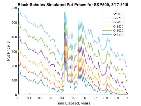
Using the solution to the Black-Scholes equation, we can simulate the price of a call or put contract expiring on Sept 1, 2018 with various strike prices, starting a year before that on Sept 1, 2017. matlab code used for the approximation is shown below:
function bs
K = 2600:100:3100; %strike prices
n = numel(K);
sigma = xlsread('VIX','sheet'); % volatility
S = xlsread('SP500','sheet');

% Call prices
figure
hold on
for i = 1:n
  cblackscholes(K(i), false,sigma,S)
end
labels('Call');
legend('location','NorthWest')

% Put prices
figure
hold on
for i = 1:n
  cblackscholes(K(i), true,sigma,S)
end
labels('Put');
end

function cblackscholes(K,isput,sigma,S)
% constants
r = 0.02; % risk free interest rate
T = 1; % day
n = length(S);
t = linspace(0,1,n);
call(n) = 0; % memory allocation
for i = 1:n
  tau = T - t(i);
  d1 = 1/(sigma(i)*sqrt(tau))*(log(S(i)/K) + (r + sigma(i)^2/2)*tau);
  d2 = d1 - sigma(i)*sqrt(tau);
  call(i) = N(d1)*S(i) - N(d2)*K*exp(-r*tau); % Black-Scholes forumla
  if isput
    call(i) = call(i) - S(i) + K*exp(-r*tau);
  end
end
plot(t,call)

end

function wt = N(d) % CDF of normal distribution
pd = makedist('Normal'); % Make probability distribution
wt = cdf(pd,d);
end

function labels(cp)
legend('K=2600','K=2700','K=2800','K=2900','K=3000','K=3100')
xlabel('Time Elapsed, years')
ylabel([cp,' Price, $'])
title(['Black-Scholes Simulated ',cp,' Prices for S&P500, 8/17-8/18'],'fontsize',12)
hold off
end
 |
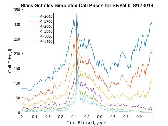 |
| Black Scholes simulated Put Prices S&P500 8/17--8/18 | Black Scholes simulated Call Prices S&P500 8/17--8/18 |
- Black, Fischer and Scholes, Myron (1973). "The Pricing of Options and Corporate Liabilities". Journal of Political Economy. 81 (3): 637--654. doi: 10.1086/260062
- Bodie, Zvi, Kane, Alex, and Marcus, Alan, Investments, 11th Edition, McGraw-Hill Education, 2018.
- Dunbar, Steven R., Solution of the Black-Scholes Equation, Stochastic Processes and Advanced Mathematical Finance.
- Esekon, Joseph Eyang’an, Analytic solution of a nonlinear Black--Scholes equation, International Journal of Pure and Applied Mathematics, Volume 82 No. 4 2013, 547--555.
- Evans, Lawrence, An Introduction to Stochastic Differential Equations, Version 1.2, Department of Mathematics of UC Berkeley. Berkeley, CA.
- Hull, John C. (1997). Options, Futures, and Other Derivatives. Prentice Hall. ISBN 0-13-601589-1.
- Kumar, S, Yildirim, A, Khan, Y, Jafari, H, Sayevand, K, and Wei, L, Analytical solution of fractional Black--Scholes European option pricing equation by using Laplace transform, ournal of Fractional Calculus and Applications, Vol. 2. Jan 2012, No. 8, pp. 1-9. ISSN: 2090-5858. http://www.fcaj.webs.com/
- Manafian, Jalil and Paknezhad, Mahnaz, Analytical solutions for the Black--Scholes equation, Applications and Applied Mathematics: An International Journal, Vol. 12, Issue 2, (December 2017), pp. 843--852.
- Merton, Robert C. (1973). "Theory of Rational Option Pricing". Bell Journal of Economics and Management Science. The RAND Corporation. 4 (1): 141–183. doi: 10.2307/3003143.
- Stecher, Michael, Converting the Black-Scholes PDE to the heat equation
- Stehlíková, Beáta, Black-Scholes model: Derivation and solution
- Yalincak, Orhun Hakan. Criticism of the Black-Scholes Model: But Why is It Still Used?: (The Answer is Simpler than the Formula). New York University. New York, NY, 2005.