Complex numbers were introduced by the Italian famous gambler and mathematician Gerolamo Cardano (1501--1576) in
1545 while he found the explicit formula for all three roots of a cube equation. Many mathematicians contributed to
the full development of complex numbers. The rules for addition, subtraction, multiplication, and division of complex
numbers were developed by the Italian mathematician Rafael Bombelli (baptized on 20 January 1526; died 1572).
The notations 1 and i for unit vectors in horizontal positive direction and
vertical positive direction, respectively, were introduced by Leonhard Euler (1707--1783) who visualized complex numbers
as points with rectangular coordinates, but did not give a satisfactory foundation for complex numbers theory. He also
suggested to drop the unit vector 1 in presenting vectors on the plane. It was Carl Friedrich Gauss
(1777--1855) who introduced the term complex number. Cauchy, a French contemporary of Gauss, extended the concept of complex numbers to the notion of complex functions.
Professor Orlando Merino (born in 1954) from the University of Rhode Island
has written an essay on the
history
of the discovery of complex numbers.
Complex numbers can be identified with three sets: the set of points on the plane (denoted by ℝ²), set of all (free) vectors on the plane, and the set of all ordered pairs of real numbers z = (x,y).
In the latter set, the first coordinate of z = (x,y) is denoted by ℜz = x (or Rez) and is called, for
historical reasons, the real part of complex number z, while the second
coordinate is denoted by ℑ ℜz = y (or Imzz. A geometric plot of complex numbers
as points z = x + jy using the x-axis as
the real axis and y-axis as the imaginary axis is referred to as an
Argand diagram.
This geometric plot is named after Jean-Robert Argand (1768–1822), who introduced it in 1806, although it was first described by Norwegian–Danish land surveyor and mathematician Caspar Wessel (1745–1818).
The set of complex numbers is one of the three sets above equipped with
arithmetic operations (addition, subtraction, multiplication, and division)
that satisfy the usual axioms of real numbers. While addition and subtraction are
inherited from vector algebra, multiplication and division satisfy specific
rules based on the identity j² = -1.
For a long time it was thought that complex numbers were just toys invented and played with only by mathematicians. After all, no single quantity in the real world can be measured by an imaginary number, a number that lives only in the imagination of mathematicians. However, in 1926, Erwin Schrödinger (1887--1961) discovered that in the language of the world of the subatomic particles, complex numbers were the indispensable alphabet. Although no single measurable physical quantity corresponds to a complex number, a pair of physical quantities can be represented very naturally by a complex number. For instance, a wave, which always consists of an amplitude and a phase, begs a representation by a complex number.

|
|
vector = Graphics[{Black, Arrowheads[0.1], Thickness[0.01],
Arrow[{{0, 0}, {2, 1}}]}];
conjugate =
Graphics[{Red, Arrowheads[0.1], Thickness[0.01],
Arrow[{{0, 0}, {2, -1}}]}];
ax = Graphics[{Black, Arrowheads[0.05], Thick,
Arrow[{{0, 0}, {2.2, 0}}]}];
ay = Graphics[{Black, Arrowheads[0.05], Thick,
Arrow[{{0, -1}, {0, 1.2}}]}];
txtj = Graphics[
Text[Style["j", Bold, FontSize -> 18, Blue], {1.91, 1.06}]];
txtC = Graphics[
Text[Style["z = a+b", FontSize -> 18, Blue], {1.7, 1.06}]];
txtjc = Graphics[
Text[Style["j", Bold, FontSize -> 18, Purple], {1.82, -1.06}]];
txtCC = Graphics[
Text[Style["a-b", FontSize -> 18, Purple], {1.7, -1.06}]];
tx = Graphics[
Text[Style["Re z", Bold, FontSize -> 18, Blue], {2.02, 0.1}]];
ty = Graphics[
Text[Style["Im z", Bold, FontSize -> 18, Blue], {0.2, 1.1}]];
Show[vector, conjugate, ax, ay, txtj, txtC, txtCC, txtjc, tx, ty]
|
|
Complex number z and its conjugate.
|
|
Mathematica code
|
It is a customary to visualize a complex number as a vector, denoting its horizontal component by
Re (real part) and its vertical component by
Im (imaginary part). In Cartesian coordinates, a complex number is denoted by the ordered pair:
\[
z = (a, b) , \qquad\mbox{with} \qquad \Re z = \mbox{Re}z = a, \quad \Im z = \mbox{Im}z = b .
\]
It was
Leonhard Euler who suggested to use two unit vectors,
1 for the abscissa and
i for the ordinate, allowing him to write
\[
z = (a, b) = a\,1 + b\,i = a + b\,i ,
\]
upon dropping multiple
1. Mathematicians still follow this genius. However, in physics, engineering, and computer science, unit vectors are usually denoted by
i,
j, and
k (most likely, you met them in calculus).
Then on the plane, a complex number can be written as
\[
z = (a, b) = a + b\,{\bf j} = a + {\bf j}\,b ,\qquad\mbox{with} \qquad \Re z = \mbox{Re}z = a, \quad \Im z = \mbox{Im}z = b .
\]
In what follows, we use
j as a unit vector in the positive vertical direction and call it the
imaginary unit. A complex number can also be written in polar form
\[
z = (a, b) = a + b\,{\bf j} = r\,e^{{\bf j}\theta} , \qquad r = \sqrt{x^2 + b^2}.
\]
Angle θ is measured in counterclockwise direction from the real axis. The complex form is based on Euler's formula:
\begin{equation} \label{EqComplex.1}
e^{{\bf j} \theta} = \cos\theta + {\bf j}\,\sin\theta .
\end{equation}
Given the complex number
z = 𝑎 +
b j, its
complex conjugate, denoted either with an overline (in mathematics) or with an asterisk (in physics and engineering), is the complex number reflected across the real axis:
\[
z^{\ast} = (a + b\,{\bf j})^{\ast} = \overline{z} = \overline{a + b\,{\bf j}} = a - b\,{\bf j} = r\, e^{-{\bf j}\theta} , \qquad \mbox{for}\quad z = r\,e^{{\bf j}\theta} .
\]
Now we are ready to define the field of complex numbers, denoted by ℂ.
The field of complex numbers, denoted by ℂ, is the set of all ordered pairs of real numbers together with the following arithmetic operations.
-
Addition: z₁ + z₂ = (x₁ + y₁ j) + (x₂ + y₂ j) = x₁ + x₂ + j (y₁ + y₂).
-
Substraction: z₁ − z₂ = (x₁ + y₁ j) − (x₂ + y₂ j) = x₁ − x₂ + j (y₁ − y₂).
-
Multiplication: z₁ ⋅ z₂ = (x₁ + y₁ j) ⋅ (x₂ + y₂ j) = (x₁x₂ − y₁y₂) + j (x₁y₂ + x₂y₁).
-
Division: division of two complex numbers z₁ ⁄ z₂ = (x₁ + y₁ j) ÷ (x₂ + y₂ j) is
\[
\frac{x_1 + {\bf j}\,y_1}{x_2 + {\bf j}\,y_2} = \frac{x_1 x_2 + y_1 y_2}{x_2^2 + y_2^2} + {\bf j}\,\frac{x_2 y_1 - x_1 y_2}{x_2^2 + y_2^2}.
\]
From the multiplication axiom, it immediately follows that
j² = −1.
Multiplication and division have extremely simple form when polar form is employed. Suppose we need to multiply two complex numbers
\[
z= r\,e^{{\bf j}\,\theta} \qquad \mbox{and} \qquad w = R\,e^{{\bf j}\,\alpha} \qquad \Longrightarrow \qquad z\cdot w = r\,R\,e^{{\bf j}\left( \theta + \alpha \right)} .
\]

|
|
vector = Graphics[{Black, Arrowheads[0.1], Thickness[0.01],
Arrow[{{0, 0}, {2, 1}}]}];
vec2 = Graphics[{Black, Arrowheads[0.1], Thickness[0.01],
Arrow[{{0, 0}, {0.7, 1}}]}];
vec = Graphics[{Black, Arrowheads[0.1], Thickness[0.01],
Arrow[{{0, 0}, {-0.6, 1.7}}]}];
ax = Graphics[{Black, Arrowheads[0.05], Thick,
Arrow[{{0, 0}, {2.2, 0}}]}];
aarr = Show[
ParametricPlot[#[[1]]*{Cos[\[Theta]],
Sin[\[Theta]]}, {\[Theta], #[[2]], #[[3]]}, Axes -> False,
PlotStyle -> #[[4]]] /.
Line[x_] :>
Sequence[Arrowheads[{-0.05, 0.05}], Arrow[x]] & /@ {{0.9,
0 Degree, 54 Degree, Red}, {1.25, 0 Degree, 27 Degree,
Blue}, {1.5, 0 Degree, 109 Degree, Green}}, PlotRange -> All]
txz = Graphics[
Text[Style["\[Theta]", FontSize -> 18, Blue], {1.6, 0.4}]];
txw = Graphics[
Text[Style["\[Alpha]", FontSize -> 18, Blue], {0.8, 0.7}]];
txzw = Graphics[
Text[Style["\[Theta] + \[Alpha]", FontSize -> 18, Blue], {0.8,
1.26}]];
Show[vector, vec2, vec, ax, aarr, txz, txw, txzw]
|
|
Multiplication of two complex numbers.
|
|
Mathematica code
|
This also allows us to easily find all roots of any complex number. Suppose that we want to calculate the n roots of a complex number
\( z = r\,e^{{\bf j}\,\theta} = r \left( \cos\theta + {\bf j}\,\sin\theta \right) . \) Then all n roots are determined from the formula:
\[
z^{1/n} = \left( r\,e^{{\bf j}\,\theta} \right)^{1/n} = \left\{ \sqrt[n]{r} \left( \cos \frac{\theta + k\,2\pi}{n} + {\bf j}\,\sin \frac{\theta + k\,2\pi}{n} \right) \right\} , \qquad k=0,1,2,\ldots , n-1.
\]
Example 1:
Let us consider the complex number 4 + 3 j that we represent in polar form
\[
4 + 3\,{\bf j} = 5\,e^{{\bf j}\,\theta} , \qquad \mbox{where}\quad \theta = \arctan \frac{3}{4} \approx 0.643501 .
\]
N[ArcTan[3/4]]
0.643501
If we want to find all three cubic roots, we need to know the angles:
N[ArcTan[3/4]/3]
0.2145
N[(2*Pi + ArcTan[3/4])/3]
2.3089
N[(4*Pi + ArcTan[3/4])/3]
4.40329
Since
N[5^(1/3)]
1.70998
we find all three cubic roots:
\[
\left( 4 + 3\,{\bf j} \right)^{1/3} \approx 1.70998 \left( \cos 0.2145 + {\bf j}\,\sin 0.2145 \right) =\approx 1.67079 + {\bf j}\,0.363984 .
\]
N[5^(1/3)]*Cos[ArcTan[3/4]/3]
1.67079
\[
\left( 4 + 3\,{\bf j} \right)^{1/3} \approx 1.70998 \left( \cos 2.3089 + {\bf j}\,\sin 2.3089 \right) =\approx -1.15061 + {\bf j}\, 1.26495.
\]
N[5^(1/3)]*Sin[(2*Pi + ArcTan[3/4])/3]
1.26495
\[
\left( 4 + 3\,{\bf j} \right)^{1/3} \approx 1.70998 \left( \cos 4.40329 + {\bf j}\,\sin 4.40329 \right) =\approx -0.520175 - {\bf j}\,1.62894 .
\]
N[5^(1/3)]*Cos[(4*Pi + ArcTan[3/4])/3]
-0.520175
Since there is no universal notation for a unit vector in vertical direction on the complex plane,
matlab uses two of them:
i and
j. Euler suggested to use
i (
\( {\bf i}^2 =-1 \) ) , so mathematicians follow him; however, in engineering and computer science it is common to use
j (
\( {\bf j}^2 =-1 \) ) .
i -- a unit imaginary vector in Mathematics, denoted by \[ImaginaryI] in Wolfram language
j -- a unit imaginary vector in Engineering and Computer Science, denoted by \[ImaginaryJ] in Wolfram language
There is no universal notation for a unit vector in a positive vertical direction on the complex plane ℂ.
Complex numbers, whose set is denoted by ℂ, have the form
\( z = x+{\bf i}y, \) or \( z = x+{\bf j}y, \)
where i, also denoted as j, is the imaginary unit
vector on the complex plane ℂ, in a positive vertical direction; so
j² = -1. matlab utelizes both standard notations
for such unit vector on complex plane: 1i and 1j. The real and imaginary parts of z are denoted as Re(z) or ℜz and Im(z) or ℑz, respectively. Unless redefined otherwise, matlab variables i as well as j denote
the imaginary unit. To introduce a complex number with real part x and
imaginary part y, one can just write x+i*y or x+1j*y; as an alternative, one can
use the command complex: complex(x,y).
Another way to define complex numbers:
matlab can handle complex numbers. Try the following
So we get the real part, the imaginary part, and the complex conjugate
\( \overline{z} = x-{\bf j}y , \)
which is also denoted in physics as
\( \overline{z} = z^{\dagger} . \) We can also get
for free its argument (angle in polar form) and the magnitude (length):
The trigonometric representations of a complex number
z is due to the Euler formula:
\[
z = \rho \,e^{{\bf j}\theta} = \rho \left( \cos\theta + {\bf j} \sin\theta \right) ,
\]
where
\( \rho = \sqrt{x^2 + y^2} \) is the modulus of the complex number (it can be obtained
by setting abs(z)) while
\( \theta \) is its argument, that is the angle between the
x axis and the straight line issuing from the origin and passing from the
point of coordinate (x, y) in the complex plane
\( \theta \) can be found by typing
angle: angle(z).
The graphical polar representation of one or more complex numbers
compass can be obtained through the command compass(z), where z is either
a single complex number or a vector whose components are complex
numbers. For instance, by typing
You can even do nasty things like
If you have not already done so, use
matlab to calculate
>> sin(pi)
ans =
1.2246e-16
The answer, of course, should be zero, but matlab returns a small, but
finite, number. This is because matlab stores floating point numbers
as sequences of binary digits with a finite length. Obviously, it is
impossible to store the exact value of "pi" in this way.
For instance, suppose we want to find all four roots of (-4)^(1/4) :
In[9]:= FullSimplify[NrootZpolar[4][-4]]
Out[9]= {1 + I, -1 + I, -1 - I, 1 - I}
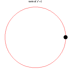
The following animation, developed by Wolfram Research, shows all
n-th roots of unity
\( \left( 1 \right)^{1/n} = \sqrt[n]{1} \) for different positive integer values of
n:
\( n=1,2,\ldots , 14 . \)
We present the following code to find and plot all roots on the complex plane:
rootPlot[equation_, variable_ : x, opts___] :=
Module[{nSol, list}, nSol = NSolve[equation, variable];
list = {Re[x], Im[x]} /. nSol;
Return[ListPlot[list, PlotStyle -> PointSize[0.03], opts]];]
The 3 underscores allows opts to match any sequence of zero or more
Mathematica expressions.
Now we plot all fifteen roots of 1:
rootPlot[x^(15) - 1 == 0, x, AspectRatio -> 1]
Another code for all roots of 1:
ShowNRoots[n_] := Module[{\[Omega] = Cos[2*Pi/n] + \[ImaginaryJ]*Sin[2*Pi/n]},
CPlot[Table[\[Omega]^k , { k, 0, n-1}]]];
ShowNRoots[9]
An elegant way of understanding the behavior of roots is to consider a root of
z as
z wanders through
the complex plane
\( \mathbb{C} . \) We shall do this by just plotting either the real part
or the imaginary part of the
n-th root of
z as
z varies in a disc around the origin. In polar coordinates, we get a function
\[
\mbox{Real part}(t, \theta ) = r^{1/n} \cos \left( \frac{\theta + t\,2\pi}{n} \right) , \qquad\mbox{or} \qquad
\mbox{Imaginary part}(t, \theta ) = r^{1/n} \sin \left( \frac{\theta + t\,2\pi}{n} \right) , \quad t=0,1,\ldots , n-1.
\]
CPlot[z_List] :=
Module[{r}, r = Map[{Re[#], Im[#]} &, z];
ListPlot[r, PlotStyle -> PointSize[0.1], AspectRatio ->1,
PlotRange -> {{-1.1, 1.1}, {-1.1, 1.1}},
PlotRegion -> {{0.05, 0.95}, {0.05, 0.95}}]]
We plot three cube roots of unity
omega = (-1 + I*Sqrt[3])/2
CPlot[{1, omega, omega^2}]