Although determination of convolution of two functions is an ill-posed problem, it sometimes can be successfully used to find the inverse Laplace transform of the image-function that is a product of two fractions. This property will be used to determine solutions of inhomogeneous differential equations and corresponding Green's functions. Therefore, this section gives an introduction to the topic, and you will see further applications in the following sections.
Definition:
If functions
f and
g are piecewise continuous on
\( [0, \infty ) , \)
then the integral
\begin{equation} \label{EqConv.1}
\left( f*g \right) (t) = g*f (t) = \int_0^{t} f(\tau )\, g(t-\tau )\, {\text d}\tau = \int_0^{t} g(\tau )\, f(t-\tau )\, {\text d}\tau
\end{equation}
is called the
convolution of
f and
g and is denoted by
\( f*g (t) . \)
Evaluation of a convolution belongs to the class of ill-posed problems. Therefore, its numerical implementation may lead to an instability.
Theorem 1:
If
f and
g are piecewise continuous on [0, ∞),
and of exponential order, then
\begin{equation} \label{EqConv.2}
{\cal L} \left[ f*g \right] (\lambda ) = {\cal L} \left[ g \right] {\cal L} \left[ f \right] = f^L \, g^L = g^L \, f^L .
\end{equation}
Application of the Laplace transformation to the convolution integral \eqref{EqConv.2} yields
\[
{\cal L} \left[ f*g \right] (\lambda ) = \int_0^{\infty} e^{-\lambda t} {\text d} t \int_0^{t} f(\tau )\, g(t-\tau )\, {\text d}\tau .
\]
Reversing the order of integration gives
\[
{\cal L} \left[ f*g \right] (\lambda ) = \int_0^{\infty} {\text d}\tau .f(\tau ) \, e^{-\lambda \tau} \int_{\tau}^{\infty} {\text d} t\,g(t-\tau )\, e^{-\lambda (t- \tau )}
\]
Substitution
u =
−τ shows that
\[
{\cal L} \left[ f*g \right] (\lambda ) = \int_0^{\infty} {\text d}\tau .f(\tau ) \, e^{-\lambda \tau} \int_{0}^{\infty} {\text d} u\, g(u) \, e^{-\lambda u} = f^L \cdot g^L .
\]
To finish the proof, we need to show that the convolution is a function-original.
The convolution theorem can be used to provide a formula for the solution of an initial value problem for a linear constant coefficient differential equation in which the forcing function is complicated to determine its Laplace transform.
Example 1:
Evaluate the Laplace transform of the convolution integral
\[
{\cal L} \left[ \int_0^t {\text d} \tau\, e^{3\tau} \,\cos \left( t- \tau \right) \right] .
\]
With
\( f(t) = e^{3t} \) and
\( g(t) = \cos t , \) the
convolution theorem states that the Laplace transform of the convolution of
f and
g is the product of
their Laplace transforms:
\[
{\cal L} \left[ \int_0^t {\text d} \tau\, e^{3\tau} \,\cos \left( t- \tau \right) \right] = {\cal L} \left[ f \right]
{\cal L} \left[ g \right] = f^L \cdot g^L .
\]
The Laplace transform of each multiple is known from the table
\begin{align*}
{\cal L} \left[ f \right] &= {\cal L} \left[ e^{3t} \right] = \frac{1}{\lambda -3} ,
\\
{\cal L} \left[ g \right] &= {\cal L} \left[ \cos t \right] = \frac{\lambda}{\lambda^2 +1} .
\end{align*}
Therefore,
\[
{\cal L} \left[ \int_0^t {\text d} \tau\, e^{3\tau} \,\cos \left( t- \tau \right) \right] =
\frac{1}{\lambda -3} \, \frac{\lambda}{\lambda^2 +1} .
\]
Now we check our calculation by explicitly evaluating the convolution integral
\[
\int_0^t {\text d} \tau\, e^{3\tau} \,\cos \left( t- \tau \right) = \frac{1}{10} \left( 3\, e^{3t} -3\,\cos t + \sin t \right) ,
\]
and then apply the Laplace transformation for every term
\[
\frac{1}{10} \,{\cal L} \left[ 3\, e^{3t} -3\,\cos t + \sin t \right] =
\frac{1}{10} \left( \frac{3}{\lambda -3} - \frac{3\,\lambda}{\lambda^2 +1} + \frac{1}{\lambda^2 +1} \right) =
\frac{3\,(\lambda^2 +1) + (1-3\lambda)(\lambda -3)}{10\,(\lambda -3)(\lambda^2 +1)} = \frac{\lambda}{(\lambda -3)(\lambda^2 +1)} .
\]
■
Example 2:
For positive numbers 𝑎 and b, evaluate
\[
{\cal L}^{-1} \left[ \frac{1}{\lambda^2 + a^2} \, \frac{1}{\lambda^2 + b^2} \right] .
\tag{2.1}
\]
Let
\[
f^L (\lambda )= \frac{1}{\lambda^2 + a^2} \qquad\mbox{and} \qquad g^L (\lambda ) = \frac{1}{\lambda^2 + b^2}
\tag{2.2}
\]
be Laplace transforms so that
\[
f (t )= {\cal L}^{-1} \left[ \frac{1}{\lambda^2 + a^2} \right] = \frac{1}{a}\, \sin at \qquad\mbox{and} \qquad
g (t ) = {\cal L}^{-1} \left[ \frac{1}{\lambda^2 + b^2} \right] = \frac{1}{b}\, \sin bt .
\tag{2.3}
\]
In this case, the convolution theorem gives
\[
{\cal L}^{-1} \left[ \frac{1}{\lambda^2 + a^2} \, \frac{1}{\lambda^2 + b^2} \right] = \frac{1}{ab} \, \int_0^t
{\text d}\tau \, \sin a\tau \,\sin b(t-\tau ) .
\]
With the aid of the trigonometric identity
\[
\sin A\,\sin B = \frac{1}{2} \left[ \cos \left( A - B \right) - \cos \left( A + B \right) \right]
\]
and the substitution
\( A = a\tau \quad\mbox{and} \quad B= b(t-\tau ) , \) we can carry out the integration
\begin{align*}
{\cal L}^{-1} \left[ \frac{1}{\lambda^2 + a^2} \, \frac{1}{\lambda^2 + b^2} \right] &= \frac{1}{ab} \, \int_0^t
{\text d}\tau \, \sin a\tau \,\sin b(t-\tau )
\\
&= \frac{1}{2ab} \, \int_0^t {\text d}\tau \left[ \cos \left( a\tau + b \tau -bt \right) - \cos \left( a\tau - b \tau +bt \right) \right]
\\
&= \frac{1}{2ab} \left[ \left. \frac{1}{a+b} \,\sin \left( a\tau + b \tau -bt \right) \right\vert_{\tau =0}^{\tau =t} -
\left. \frac{1}{a-b} \, \sin \left( a\tau - b \tau +bt \right) \right\vert_{\tau =0}^{\tau =t} \right]
\\
& \quad \\
&= \left[ \frac{\sin at + \sin bt}{2(a+b)ab} - \frac{\sin at - \sin bt}{2(a-b)ab} \right] H(t) , \tag{2.4}
\end{align*}
where
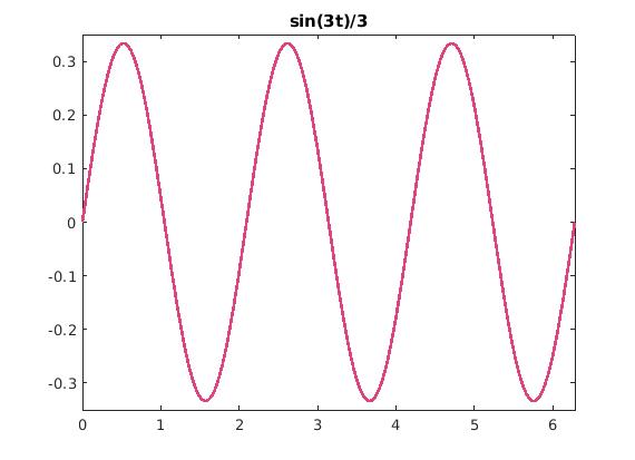
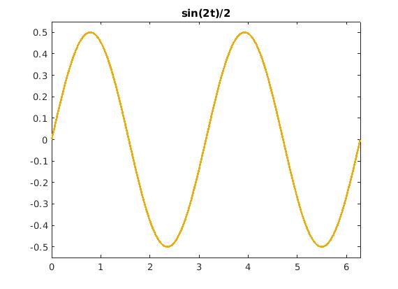
H(t) is the Heaviside function. Let us make a numerical experiment and set 𝑎 = 3 and
b = 2. Then
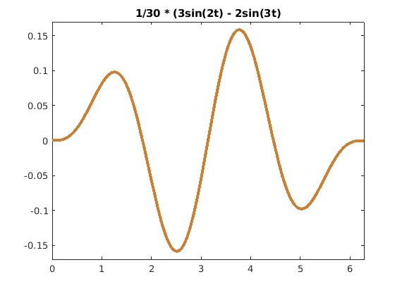
\[
\frac{\sin 3t}{3} \ast \frac{\sin 2t}{2} = \frac{\sin 2t}{2} \ast \frac{\sin 3t}{3} = \frac{1}{6} \int_0^t \sin 3(t-\tau )\,\sin 2\tau \,{\text d}\tau = \frac{1}{30}\left( 3\,\sin 2t - 2\,\sin 3t \right) H(t) .
\]
We verify the integration and plot these functions with
matlab:
syms t s
int(sin(3*t - 3*s) * sin(2*s), s, [0 t])

fplot(sin(3*t)/3, [0, 2*pi], 'color', [0.88 0.26 0.5], 'LineWidth', 2)
title('sin(3t)/3')
ylim([-0.35, 0.35])

fplot(sin(2*t)/2, [0, 2*pi], 'color', [0.93 0.68 0.05], 'LineWidth', 2)
title('sin(2t)/2')
ylim([-0.55, 0.55])

fplot(1/30 * (3*sin(2*t) - 2*sin(3*t)), [0, 2*pi], 'color', [0.8 0.5 0.2], 'LineWidth', 2)
title('1/30 * (3sin(2t) - 2sin(3t)')
ylim([-0.17, 0.17])

fplot(1/6 *sin(2*t)*sin(3*t), [0, 2*pi], 'color', [0.8 0.5 0.2], 'LineWidth', 3)
title('Product sin(2t) sin(3t)/6')
ylim([-0.17, 0.17])
>> ans =
(3*sin(2*t))/5 - (2*sin(3*t))/5
|
|
|
|
|
|
|
|
sin(3t)/3
|
|
sin(2t)/2
|
|
Convolution of sin(2t)/2 and sin(3t)/3.
|
|
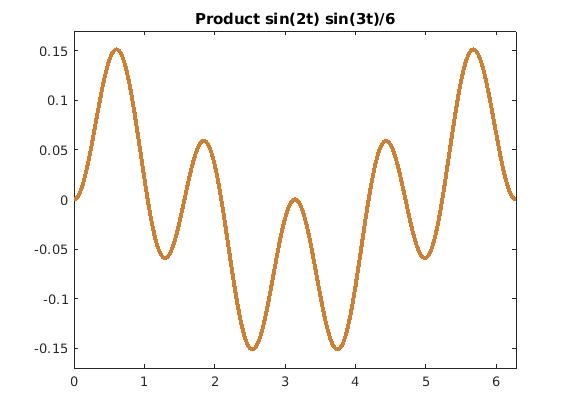
Product of sin(2t)/2 and sin(3t)/3.
|
To check the answer (2.4), we apply the Laplace transform to the right-hand side:
\[
{\cal L} \left[ \frac{\sin at + \sin bt}{2(a+b)ab} - \frac{\sin at - \sin bt}{2(a-b)ab} \right] = \frac{1}{\lambda^2 + a^2}
\left[ \frac{1}{2(a+b)b} - \frac{1}{2(a-b)b} \right] + \frac{1}{\lambda^2 + b^2} \left[ \frac{1}{2(a+b)a} + \frac{1}{2(a-b)a} \right] .
\]
Since
\[
\frac{1}{2(a+b)b} - \frac{1}{2(a-b)b} = - \frac{1}{a^2 - b^2} \qquad\mbox{and} \qquad \frac{1}{2(a+b)a} + \frac{1}{2(a-b)a} = \frac{1}{a^2 - b^2} ,
\]
we have
\[
{\cal L} \left[ \frac{\sin at + \sin bt}{2(a+b)ab} - \frac{\sin at - \sin bt}{2(a-b)ab} \right] = \frac{1}{a^2 - b^2}
\ \left( \frac{-1}{\lambda^2 + a^2} + \frac{1}{\lambda^2 + b^2} \right) = \frac{1}{\lambda^2 + a^2} \, \frac{1}{\lambda^2 + b^2} .
\]
■
Example 3:
Solve the integral equation
\[
y(t) = 3t^2 - e^{-2t} + \int_0^t y(\tau ) \, e^{2t-2\tau}\, {\text d}\tau
\tag{3.1}
\]
for
y(t).
We identify the integral in the right-hand side as the convolution of unknown function and the exponential function.
We take the Laplace transform of each term:
\[
{\cal L} \left[ y \right] = y^L = {\cal L} \left[ 3t^2 \right] - {\cal L} \left[ e^{-2t} \right] + {\cal L} \left[ \int_0^t y(\tau ) \, e^{2t-2\tau}\, {\text d}\tau \right]
\]
We denote by
\( y^L = \int_0^{\infty} y(t)\, e^{\lambda\,t} \,{\text d}t \) the Laplace transform of unknown function. Then
\begin{align*}
{\cal L} \left[ 3t^2 \right] &= \frac{6}{\lambda^3} ,
\\
{\cal L} \left[ e^{-2t} \right] &= \frac{1}{\lambda +2} ,
\\
{\cal L} \left[ \int_0^t y(\tau ) \, e^{2t-2\tau}\, {\text d}\tau \right] &= y^L \,{\cal L} \left[ e^{2t} \right]
= y^L \,\frac{1}{\lambda -2} .
\end{align*}
Therefore, upon application of the Laplace transform, we get an algebraic equation instead of an integral equation:
\[
y^L = \frac{6}{\lambda^3} - \frac{1}{\lambda +2} + y^L \,\frac{1}{\lambda -2} .
\]
Solving for
yL, we obtain
\[
y^L = \frac{\lambda -2}{\lambda -3} \left( \frac{6}{\lambda^3} - \frac{1}{\lambda +2} \right) .
\]
Now applying the inverse Laplace transform to the right-hand side expression, we get the required solution
syms t s
ilaplace((s - 2)/(s - 3)*(6/s^3 - 1/(s + 2)), s, t)
>> ans =
exp(3*t)/45 - (4*exp(-2*t))/5 - (2*t)/3 + 2*t^2 - 2/9
\[
y(t) = \left[ \frac{2}{9} \left( 9t^2 -3t-1 \right) + \frac{1}{45}\, e^{3t} - \frac{4}{5}\, e^{-2t} \right] H(t) .
\]
■
Example 4:
Determine the current i(t) in a single-loop LRC circuit when
L = 0.5 henries, R = 3 ohms, C = 0.2 farads, i(0) = 0, and the impressed voltage is
\[
E(t) = 127\,t - 127\,t\, H(t-\pi ) .
\]
In a single-loop circuit, Kirchhoff's second law states that the sum of the voltage drops across an inductor,
resistor, and capacitor is equal to the impressed voltage
E(
t). Then current
i(
t) is governed by the
integrodifferential equation
\[
L\, \frac{{\text d}i}{{\text d}t} + R\, i(t) + \frac{1}{C} \, \int_0^t i(\tau )\,{\text d}\tau = E(t) .
\]
Substituting the given values, we obtain the initial value problem for the integrodifferential equation:
\[
0.5\, \frac{{\text d}i}{{\text d}t} + 3\, i(t) + 5 \, \int_0^t i(\tau )\,{\text d}\tau = 127\,t - 127\,t\, H(t-\pi ) , \qquad i(0) =0.
\]
Application of the Laplace transform to the above problem yields
\[
0.5\, \lambda\, i^L + 3\, i^L + 5 \, i^L \, \frac{1}{\lambda} = E^L = \frac{127}{\lambda^2} \left( 1 - e^{-\lambda\pi} \right)
- \frac{127\,\pi}{\lambda} \, e^{-\lambda\pi} .
\]
Solving with respect to the Laplace transform of the unknown current
iL, we obtain
\[
i^L (\lambda ) = \frac{2\lambda}{\lambda^2 +6\lambda +10}\, E^L = \frac{254}{\lambda^2 +6\lambda +10} \left[ \frac{1}{\lambda} -
\frac{1}{\lambda} \,e^{-\lambda\pi} - \pi\, e^{-\lambda\pi} \right]
\]
To determine the current through this application of the inverse Laplace transform, we introduce two functions
\[
f^L (\lambda ) = \frac{254}{\lambda \left( \lambda^2 +6\lambda +10\right)}\qquad\mbox{and} \qquad
g^L (\lambda ) = \frac{254}{\lambda^2 +6\lambda +10} .
\]
Then the required current will be equal to
\[
i(t) = f(t) - f(t-\pi ) - \pi\,g(t-\pi ) ,
\]
where functions
f and
g are defined by the inverse Laplace transforms:
\begin{align*}
f(t) &= {\cal L}^{-1} \left[ \frac{254}{\lambda \left( \lambda^2 +6\lambda +10\right)} \right] ,
\\
g(t) &= {\cal L}^{-1} \left[ \frac{254}{\lambda^2 +6\lambda +10} \right] .
\end{align*}
The denominator in both expressions contains the polynomial
\( Q(\lambda ) = \lambda^2 +6\lambda +10 \) that has two complex conjugate nulls:
\( \lambda = -3 \pm {\bf j} . \) Applying the residue method, we find
\[
g(t) = 2\,\mbox{Re} \,\mbox{Res}_{\lambda = -3 + {\bf j}} \, \frac{254}{\lambda^2 +6\lambda +10} \, e^{\lambda \,t} .
\]
The residue is
\[
\mbox{Res}_{\lambda = -3 + {\bf j}} \, \frac{254}{\lambda^2 +6\lambda +10} \, e^{\lambda \,t} = \left. \frac{254}{2\lambda +6} \, e^{\lambda\, t} \right\vert_{\lambda = -3 + {\bf j}}
= \frac{127}{\bf j} \, e^{-3t} \, e^{{\bf j} t}.
\]
Extracting the real part, we get
\[
g(t) = 254\,e^{-3t} \,\sin t \, H(t) ,
\]
where
H(
t) is the Heaviside function. To determine the inverse Laplace transform of the function
\( f^L (\lambda ) , \) we need to calculate two residues, at λ = 0 and at λ = -3 +
j.
This leads to
\begin{align*}
\mbox{Res}_{\lambda = -3 + {\bf j}} \, \frac{254}{\lambda \left( \lambda^2 +6\lambda +10 \right)} \, e^{\lambda \,t} &=
\lim_{\lambda \mapsto -3 + {\bf j}} \, \frac{127}{\lambda \left( \lambda +3 \right)} \, e^{\lambda \,t}
= - \frac{127}{1 + 3{\bf j}} \,e^{-3t} \, e^{{\bf j} t}
\\
\mbox{Res}_{\lambda = 0} \, \frac{254}{\lambda \left( \lambda^2 +6\lambda +10 \right)} \, e^{\lambda \,t} &=
\lim_{\lambda \mapsto 0} \, \frac{254}{\lambda^2 +6\lambda +10} \, e^{\lambda \,t} = \frac{127}{5} .
\end{align*}
Extracting the real part, we get
\[
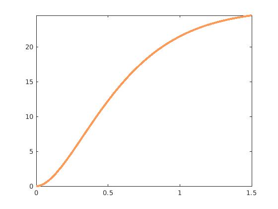
f(t) = \left[ \frac{127}{5} - \frac{127}{5}\,e^{-3t} \left( 3\,\sin t + \cos t \right) \right] H(t) ,
\]
|
|
We plot the solution with matlab
syms t s
fplot(127/5 - 127/5*exp(-3*t)*(3*sin(t) + cos(t)), [0, 1.5], 'color', [1 0.6 0.33], 'LineWidth', 3)
|
■