The
Heaviside function (also known as a unit step function) models the on/off behavior of a switch; e.g., when voltage is switched on or off in an electrical circuit, or when a neuron becomes active (fires). It is denote by
H(
t) according to the formula:
\begin{equation} \label{EqHeaviside.1}
H(t) = \begin{cases} 1, & \quad t > 0 , \\
1/2, & \quad t=0, \\
0, & \quad t < 0. \end{cases}
\end{equation}
|
|
|
a=1;
title(['Shifted Heaviside function H(t - a),',' a = ',num2str(a)])
hold on
plot([-a,a],[0,0],'b','linewidth',3)
plot([a,3*a],[1,1],'b','linewidth',3)
plot(a,1/2,'b.','markersize',22)
plot(a,0,'b>','markersize',10,'markerfacecolor','b')
plot(a,1,'b<','markersize',10,'markerfacecolor','b')
|
matlab® has a dedicated built-in command for the Heaviside function:
heaviside. Here are some examples how to use it:
heaviside(sym(2))
heaviside(sym(-5))
>> ans =
1/2
See the difference in output:
heaviside(sym(0))
heaviside(0)
>> ans =
0.5000
The former gives the actual value at t = 0 to be one half, although the latter gives the numerical output: 0.5000.
Although matlab® has a build-in Heaviside function, heaviside, its visualization is based on connecting the jump at the point of discontinuity.
|
|
|
syms t
fplot(heaviside(t), [-2, 2], 'linewidth',3)
|
Since
matlab® is a programming language, an endless variety of different signals is possible. For instance, we can define the unit step function as follows:
t = (-1:0.01:1)';
unitstep = t>=0;
plot(t,unitstep, LineWidth = 5)
As you see from the graphs, both functions,
heaviside and UnitStep, result in the same graph.
The Heaviside function is related to the signum function:
\[
H(t) = \frac{1}{2} \left( \mbox{sign} t + 1 \right) , \qquad\mbox{with} \quad \mbox{sign} t = \begin{cases} \phantom{-}1, & \quad t > 0 , \\
\phantom{-}0, & \quad t=0, \\
-1, & \quad t < 0. \end{cases}
\]
Then the Heaviside function can be uniquely defined as
syms t
heavi = (sign(t) + 1)/2;
plot(t, heavi, 'linewidth', 3)
Instead, we plot approximations of the Heaviside function based on its generator
\[
G(z) = \frac{-1}{2\pi\,{\bf j}}\, \ln (-z) \qquad\Longrightarrow \qquad H(t) = \lim_{\varepsilon \to 0} \left[ G\left( t + \varepsilon \right) - G\left( t - \varepsilon \right) \right] ,
\]
where
j is the unit vector in the positive vertical direction on the complex plane ℂ, so
j² = −1. We use
Chebfun and take the real part only to remove imaginary rounding errors.
|
|
|
G = @(z) -1/(2*pi*1j)*log(-z);
x = chebfun('x', [-3,3]);
hyperHeaviside = @(ep) real(G(x+1j*ep)-G(x-1j*ep));
for ep = .1:-.01:.001;
    plot(hyperHeaviside(ep), 'color', [.2 0 .7]), hold on
end
title('Heaviside function','fontsize',12), hold off
|
There are known many other
generators of the Heaviside function. For example,
\[
H\left( t \right) = \lim_{s\to\infty} \,\left[ \frac{1}{2} + \frac{1}{\pi}\,\arctan \left( st \right) \right] .
\]
The Laplace transform of the Heaviside function (as well as the UnitStep function) is
syms t
laplace(heaviside(t))
>> ans =
1/s
\begin{equation} \label{EqHeaviside.2}
{\cal L} \left[ H(t) \right] = \int_0^{\infty} 1\cdot e^{-\lambda t} {\text d}t = \frac{1}{\lambda} .
\end{equation}
By default,
matlab uses
s as output variable; however, we will use λ where possible.
We defined previously the
UnitStep:
\[
{\bf UnitStep}(t) = \begin{cases} 1, & \quad t \ge 0 , \\
0, & \quad t < 0; \end{cases}
\]
that assigns the value of 1 to
t = 0.
Its Laplace transform is the same as for the Heaviside function because
the Laplace transformation \eqref{EqHeaviside.1} does not care about values of a transformed function at discrete number of points (that should not cluster to a point). So you can define the value of the Heaviside function at t = 0 whatever you want:
\[
u(t) = \begin{cases}
1 , & \ \mbox{ for }\ t > 0,
\\
\mbox{whatever you want}, & \ \mbox{ for }\ t=0,
\\
0, & \ \mbox{ for }\ t < 0.
\end{cases}
\]
Then its Laplace transform becomes
\[
{\cal L} \left[ u(t) \right] = {\cal L} \left[ H(t) \right] = {\cal L} \left[ \mbox{UnitStep}(t) \right] = \frac{1}{\lambda} ,
\]
independently on the value of these functions at
t = 0.
However, the inverse Laplace transform restore only the Heaviside function, but not
u(
t). This is the reason why we use the definition of the Heaviside function, but any other unit step function.
\[
{\cal L}^{-1} \left[ \frac{1}{\lambda} \right] = H(t) .
\]
In the next section, we will show how the Heaviside function can be used to determine the Laplace transforms of piecewise continuous functions. The main tool
to achieve this is the shifted Heaviside function H(t−𝑎), where 𝑎 is arbitrary positive number.
We find the Laplace transform of shifted Heaviside function with the aid of
matlab
syms t lambda
syms a positive
laplace(heaviside(t-a),t,lambda)
>> ans =
exp(-a*lambda)/lambda
Its Laplace transform is
\[
\left( {\cal L} \,H(t-a) \right) (\lambda ) = \int_a^{\infty}\,e^{-\lambda t} \,{\text d} t = \frac{1}{\lambda -a}\, e^{=a\lambda} .
\]
We present a property of the Heaviside function that is not immediately obvious:
\[
H\left( t^2 - a^2 \right) = 1- H(t-a) + H(t+a) = \begin{cases} 1, & \quad t < -a , \\
0, & \quad -a < t < a, \\
1, & \quad t > a > 0. \end{cases}
\]
The most important property of shifted Heaviside functions is that their difference, W(𝑎,b) = H(t-𝑎) - H(t-b), is actually a window over the interval (𝑎,b); this means that their difference is 1 over this interval and zero outside closed interval [𝑎,b]:
|
|
|
a=2;
title(['Shifted Heaviside function H(t^2 - a^2),',...
' a = ',num2str(a)],'fontsize',14)
hold on
plot([-a,a],[0,0],'b','linewidth',3)
plot(a,0,'b>','markersize',10,'markerfacecolor','b')
plot([a,3*a],[1,1],'b','linewidth',3)
plot(a,1,'b<','markersize',10,'markerfacecolor','b')
plot(3*a,1,'b>','markersize',10,'markerfacecolor','b')
plot([a,3*a],[1/2,1/2],'b.','markersize',22)
plot([3*a,4*a],[0,0],'b','linewidth',3)
plot(3*a,0,'b<','markersize',10,'markerfacecolor','b')
|
The Laplace transform of the window function is
\[
\left( {\cal L} \,W(t; a,b) \right) (\lambda ) = \int_a^{b}\,e^{-\lambda t} \,{\text d} t = \frac{1}{\lambda}\, e^{-a\lambda} - \frac{1}{\lambda}\, e^{-b\lambda} .
\]
syms t a b
a = 2;
b = 3;
laplace(heaviside(t - a) - heaviside(t - b))
>> ans =
exp(-2*s)/s - exp(-3*s)/s
Example 1:
Consider the piecewise continuous function
\[
f(t) = \begin{cases} 1, & \quad 0 < t < 1 , \\
t, & \quad 1 < t < 2 , \\
t^2 , & \quad 2 < t < 3 , \\
0, & \quad 3 < t . \end{cases}
\]
Of course, we can find its Laplace transform directly
\[
f^L (\lambda ) = \int_0^{\infty} f(t)\,e^{-\lambda \,t} \,{\text d} t = \int_0^{1} \,e^{-\lambda \,t} \,{\text d} t + \int_1^{2} t \,e^{-\lambda \,t} \,{\text d} t
+ \int_2^{3} t^2 \,e^{-\lambda \,t} \,{\text d} t .
\]
However, we can also find its Laplace transform using the shift rule. First, we represent the given function
f(t) as the sum
\[
f(t) = H(t) - H(t-1) + t \left[ H(t-1) - H(t-2) \right] + t^2 \left[ H(t-2) - H(t-3) \right] .
\]
We consider each term on the right-hand side separately.
\begin{align*}
t \, H(t-1) &= (t-1+1) \, H(t-1) = \left( t-1 \right) H(t-1) + H(t-1) \qquad\Longrightarrow \qquad {\cal L} \left[ t \, H(t-1) \right] = \frac{1}{\lambda^2} \, e^{-\lambda} + \frac{1}{\lambda}\, e^{-\lambda} ,
\\
t \, H(t-2) &= \left( t-2 +2 \right) H(t-2) = \left( t-2 \right) H(t-2) + 2\, H(t-2) \qquad\Longrightarrow \qquad {\cal L} \left[ t \, H(t-2) \right] = \frac{1}{\lambda^2} \, e^{-2\lambda} + \frac{2}{\lambda}\, e^{-2\lambda} ,
\\
t^2 \, H(t-2) &= \left( t-2 +2 \right)^2 H(t-2) = \left( t-2 \right)^2 H(t-2) + 4 \left( t-2 \right) H(t-2) + 4\, H(t-2) \qquad\Longrightarrow \qquad {\cal L} \left[ t^2 \, H(t-2) \right] = \frac{2}{\lambda^3} \, e^{-2\lambda} + \frac{4}{\lambda^2}\, e^{-2\lambda} + \frac{4}{\lambda}\, e^{-2\lambda} ,
\\
t^2 \, H(t-3) &= \left( t-3 +3 \right)^2 H(t-3) = \left( t-3 \right)^2 H(t-3) + 6 \left( t-3 \right) H(t-3) + 9\, H(t-3) \qquad\Longrightarrow \qquad {\cal L} \left[ t^2 \, H(t-3) \right] = \frac{2}{\lambda^3} \, e^{-3\lambda} + \frac{6}{\lambda^2}\, e^{-3\lambda} + \frac{9}{\lambda}\, e^{-3\lambda} .
\end{align*}
Collecting all terms, we obtain
\[
f^L (\lambda ) = \frac{2}{\lambda^3} \left( e^{-2\lambda} - e^{-3\lambda} \right) + \frac{1}{\lambda^2} \left( e^{-\lambda} + 3\, e^{-2\lambda} -6\,e^{-3\lambda} \right) + \frac{1}{\lambda} \left( 1 + 2\,e^{-2\lambda} - 9\,e^{-3\lambda} \right) .
\]
The delta function, δ(
x), also called the
Dirac delta function, is an object that is not a function according to the definition given in calculus. It is a useful device that behaves in many cases as a function. We show how to use it in a heuristic and non-rigorous manner because its justification would take us far beyond the scope of this tutorial.
Paul Adrien Maurice Dirac (1902--1984) was an English theoretical physicist who made fundamental contributions to the
early development of both quantum mechanics and quantum electrodynamics.
Paul Dirac was born in Bristol, England, to a Swiss father and an English mother. Paul admitted that he had an
unhappy childhood, but did not mention it for 50 years; he learned to speak French, German, and Russian. He received
his Ph.D. degree in 1926. Dirac's work concerned mathematical and theoretical
aspects of quantum mechanics. He began work on the new quantum mechanics as soon as it was introduced by Heisenberg
in 1925 -- independently producing a mathematical equivalent, which consisted essentially of a noncommutative algebra
for calculating atomic properties -- and wrote a series of papers on the subject. Among other discoveries, he
formulated the Dirac equation, which describes the behavior of fermions and predicted the existence of antimatter.
Dirac shared the 1933 Nobel Prize in physics with
Erwin Schrödinger "for the discovery of new productive forms of
atomic theory."
Dirac had traveled extensively and studied at various foreign universities, including Copenhagen, Göttingen, Leyden, Wisconsin, Michigan, and Princeton.
In 1937 he married Margit Wigner, of Budapest. Dirac was regarded by his friends and colleagues as unusual in
character for his precise and taciturn nature. In a 1926 letter to Paul Ehrenfest,
Albert Einstein wrote of Dirac,
"This balancing on the dizzying path between genius and madness is awful." Dirac openly criticized the political
purpose of religion. He said: "I cannot understand why we idle discussing religion. If we are honest---and
scientists have to be---we must admit that religion is a jumble of false assertions, with no basis in reality."
He spent the last decade of his life at Florida State University.
The Dirac delta function was introduced as a "convenient notation" by Paul Dirac in his
influential 1930 book, "The Principles of Quantum Mechanics," which was based on his most celebrated result on
relativistic equation for electron, published in 1928. He called it the "delta function" since he used it as a
continuous analogue of the discrete
Kronecker delta \( \delta_{n,k} . \) Dirac predicted the existence of positron, which was first
observed in 1932. Historically, Paul Dirac used δ-function for modeling the density of an idealized point mass
or point charge, as a function that is equal to zero everywhere except for zero and whose integral over the entire
real line is equal to one.
As there is no function that has these properties, the computations that were done by the
theoretical physicists appeared to mathematicians as nonsense. It took a while for mathematicians to give strict
definition of this phenomenon. In 1938, the Russian mathematician Sergey Sobolev (1908--1989) showed that
the Dirac function is a derivative (in a generalized sense, also known as in a weak sense) of the Heaviside function. To define derivatives of
discontinuous functions, Sobolev introduced a new definition of differentiation and the corresponding set of generalized
functions that were later called distributions. The French mathematician Laurent-Moïse Schwartz (1915--2002) further
extended Sobolev's theory by pioneering the theory of distributions, and he was rewarded the Fields Medal in 1950 for
his work. Because of his sympathy for Trotskyism, Schwartz encountered serious problems trying to enter the United
States to receive the medal; however, he was ultimately successful. But it was news without major consequence,
for Schwartz’ work remained inaccessible to all but the most determined of mathematical physicists.
Many scientists refuse existence of the delta function and claim that all theoretical results can be obtained without it.
Dirac’s cautionary remarks (and the efficient simplicity of his idea)
notwithstanding, some mathematically well-bred people did from the outset
take strong exception to the δ-function. In the vanguard of this group was the American-Hungarian mathematician
John von Neumann (was born in Jewish family as János Neumann, 1903--1957), who dismissed the δ-function as a “fiction."
Although it is hard to argue against this point of view, applications of the Dirac delta-functions are so diverse and its convenience was shown in various examples that its usefulness is widely accepted.
Sergey Sobolev (left) and Laurent Schwartz (right).
In 1955,
the British applied mathematician George Frederick James Temple (1901--1992) published
what he called a “less cumbersome vulgarization” of Schwartz’ theory based on Jan Geniusz Mikusınski's (1913--1987)
sequential approach. However, the definition of δ-function can be traced back to the early 1820s due to the work
of Joseph Fourier on what we now know as the Fourier integrals. In 1828, the δ-function had intruded for a second time
into a physical theory by George Green who noticed that the solution to the nonhomogeneous Poisson equation
can be expressed through the solution of a special equation containing the delta function. The history of the theory
of distributions can be found in "The Prehistory of the Theory of Distributions" by Jesper Lützen (University of Copenhagen, Denmark), Springer-Verlag, 1982.
Outside of quantum mechanics the delta function is also known in engineering and signal processing as the unit
impulse symbol. Mechanical systems and electrical circuits are often acted upon by an external force of large magnitude
that acts only for a very short period of time. For example, all strike phenomenon (caused by either piano hammer or
tennis racket) involve impulse functions. Also, it is useful to consider discontinuous idealizations,
such as the mass density of a point mass, which has a finite amount of mass stuffed inside a single point of space.
Therefore, the density must be infinite at that point and zero everywhere else. Delta function can be defined as the derivative of the Heaviside function,
which (when formally evaluated) is zero for all \( t \ne 0 , \) and it is undefined at the
origin. Now time comes to explain what a generalized function or distribution means.
In our everyday life, we all use functions that we learn from school as a map or transformation of one set (usually
called input) into another set (called output, which is usually a set of numbers). For example, when we do our annual physical examinations,
the medical staff measure our blood pressure, height, and weight, which all are functions that can be described as nondestructive testing. However, not all functions
are as nice as previously mentioned. For instance, a biopsy is much less pleasant option and it is hard to call it a
function, unless we label it a destructive testing function. Before the procedure, we consider a patient as a probe function, but after biopsy when some tissue has been
taken from patient's body, we have a completely different person. Therefore, while we get biopsy laboratory results (usually represented in numeric digits), the biopsy represents destructive testing.
Now let us turn to another example. Suppose you visit a store and want to purchase a soft drink, i.e. a bottle of soda. You
observe that liquid levels in each bottle are different and you wonder whether they filled these bottles with different volumes
of soda or the dimensions of each bottle differ from one another. So you decide to measure the volume of soda in a particular bottle.
Of course, one can find outside dimensions of a bottle, but to measure the volume of soda inside, there is no
other option but to open the bottle. In other words, you have to destroy (modify) the product by opening the bottle. The function of measuring the soda by opening the bottle could represent destructive testing
Now consider an electron. Nobody has ever seen it and we do not know exactly what it looks like. However, we can make some measurements
regarding the electron. For example, we can determine its position by observing the point where electron strikes a
screen. By doing this we destroy the electron as a particle and convert its energy into visible light to determine its position in space.
Such operation would be another example of destructive testing function, because we actually transfer the electron into another matter, and we
actually lose it as a particle. Therefore, in the real world we have and use nondestructive testing functions that measure items without their
termination or modification (as we can measure velocity or voltage). On the other hand, we can measure some items only by completely destroying them or transferring them into another options as destructive testing functions. Mathematically, such measurement could be
done by integration (hope you remember the definition from calculus):
\[
\int_{-\infty}^{\infty} f(x)\,g(x)\,{\text d}x ,
\]
where
f(
x) is a nice (probe) function and
g(
x) can represent (bad or unpleasant) operation on our probe function.
As a set of probe functions, it is convenient to choose smooth functions on the line with compact support
(which means that they are zero outside some finite interval). As for an electron, we don't know what the multiple
g(
x) looks like, all we know is the value of integral that represents a measurement. In this case, we say
that
g(
x) acts on the probe function and we call this operation the
functional. Physicists denote it as
\[
\left. \left\vert g \right\vert f \right\rangle = \int_{-\infty}^{\infty} f(x)\,g(x)\,{\text d}x \qquad\mbox{or simply}
\qquad \langle g, f \rangle .
\]
(for simplicity, we consider only real-valued functions).
Mathematicians also follow these notations; however, the integral on the right-hand side is mostly a show of respect to
people who studied functions at school and it has no sense because we don't know what is the exact expression of
g(x)---all we know or measure is the result of integration. Such objects as
g(
x) are now called distributions,
or generalized functions, but actually they are all functionals:
g acts on any probe function by mapping it into
a number (real or complex). So strictly speaking, instead of the integral
\( \int_{-\infty}^{\infty} f(x)\,g(x)\,{\text d}x \) we have to write the formula
\[
g\,:\, \mbox{set of probe functions } \mapsto \, \mbox{numbers}; \qquad g\,: \, f \, \mapsto \, \mathbb{R} \quad
\mbox{or}\quad \mathbb{C} .
\]
Therefore, the notation
g(x) makes no sense because the value of
g at any point
x is undefined.
So
x is a dummy variable or invitation to consider functions depending on
x. It is
more appropriate to write
\( g(f) \) because it is a number that
is assigned to a probe function
f by distribution
g. Nevertheless, it is a custom to say that a
generalized function
g(x) is zero
for
x from some interval [a,b] if, for every probe function
f that is zero outside the given interval,
\[
\langle g , f \rangle = \int_a^b f(x)\, g(x)\, {\text d} x =0.
\]
However, it is completely inappropriate to say that a generalized function has a particular value at some point
(recall that the integral does not care about a particular value of integrable function).
Following Sobolev, we define a derivative
g' of a distribution
g by the equation
\[
\langle g' , f \rangle = -\int_a^b f'(x)\, g(x)\, {\text d} x ,
\]
which is valid for every smooth probe function
f that is identically zero outside some finite interval.
Now we define the derivative of the Heaviside function using the new definition (because the old calculus definition of a
derivative is useless).
⁎ ✱ ✲ ✳ ✺ ✻ ✼
✽ ❋ ===================================
In many application, we come across functions that have a very large value over a very short interval. For example, the strike of a hammer exerts a relatively large force over a relatively short time and a heavy weight concentration at a spot on a suspended beam exerts a large force over a very small section of the beam. A typical example of the latter is the pressure of tran's wheel on rails. To deal with impulse functions (that represent violent forces of short duration), physicists and engineers use the special notation, introduced by Paul Dirac and is called the delta function.
Definition:
The
Dirac delta function δ(
t) is a
functional that assigns to every smooth function
f ∈
S from a set of test (probe) functions
S a real (or complex) number according to the formula
\begin{equation} \label{EqDirac.1}
\langle \delta (t- t_0 ) | f(t) \rangle = \int_{-\infty}^{\infty} \delta (t- t_0 ) \, f\left( t\right) \,{\text d}t = f\left( t_0\right) .
\end{equation}
The right-hand side of Eq.\eqref{EqDirac.1} is also denoted as < δ ,
f > or simply (δ ,
f). The dimensions of δ(
t) are the inverse of the dimensions of
t because the quantity δ(
t) d
t must be dimensioness.
Now we give an explanation regarding notations.
Here we use
bra–ket notation, <
g |
f>, that was effectively established in 1939 by Paul Dirac and is thus also known as the Dirac notation. In this notation, bra <
g | represents a
functional, and ket |
f > stands for a probe function. Historically, functionals are usually identified with integrals because every quadrature
\[
F(f) = \int_a^b f(x)\,g(x)\,{\text d}x
\]
determines a
functional by assigning to every integrable function
f(
x) a number
F(
f).
A set of probe (or test) functions is usually chosen as a subset of the set C∞ of infinitely differentiable functions that approach zero at infinity to ensure that \( \int_{-\infty}^{\infty} \left\vert f (x) \right\vert^2 {\text d}x \) converges. The set of all square integrable functions is denoted by 𝔏²(ℝ) or simply 𝔏² (notations L² or L2 are also widely used). This space becomes a Hilbert space with the inner product
\begin{equation} \label{EqDirac.2}
\left\langle g(x) \,|\, f(x) \right\rangle = \left\langle g(x) , f(x) \right\rangle = (f, g) = \int_{-\infty}^{\infty} \overline{g(x)} \,f(x)\,{\text d}x
\end{equation}
that generates the
norm
\[
\| f(x) \|^2 = \left\langle f(x) , f(x) \right\rangle = (f, f) = \int_{-\infty}^{\infty} \left\vert f(x)\right\vert^2 {\text d}x .
\]
The elements of the Hilbert space 𝔏² of square integrable functions aren’t functions. They are equivalence classes of functions, where two functions belong to the same class if they are equal almost everywhere (meaning, they are unequal merely on a set of measure 0). Therefore, the element
f ∈ 𝔏²(ℝ)
doesn’t have a well-defined value anywhere: you can take any square-integrable function
f, change its value at
x=0 to be 17 or −100, and you still have the same element in 𝔏². Every functional on 𝔏² is generated by some function from itself:
\[
F(f) = \left\langle g, f \right\rangle = (g,f) ,
\]
for some function
g∈𝔏². This is the reason why an action of the delta function on a probe function is denoted by the integral \eqref{EqDirac.1}. However, a probe function
f must be at least continuous for relation \eqref{EqDirac.1} to be valid.
From the definition above, it follows that the delta function is a distribution. It turns out that the majority of usual operations of calculus are applicable to generalized functions; of course, they can be justified rigorously. Although ordinary functions can be canonically reinterpreted as acting on test functions, there are many distributions that do not arise in this way; and delta function is one of them.
There is no way to define the value of a distribution at a particular point. However, we can extend it and define, for instance, a generalized function to have zero values on some open interval. We demonstrate this concept on a particular example by calculating the derivative of the Heaviside function. To find the derivative of a distribution, we need a new definition that was first proposed by S. Sobolev, who called it weak or generalized derivative:
\[
\int g' (x)\, f(x)\,{\text d}x = - \int g(x)\,f' (x) \,{\text d} x .
\]
Example 2:
Since the Heaviside function
\[
H(x) = \begin{cases}
1, & \ \mbox{ when } x > 0, \\
1/2, & \ \mbox{ for } x = 0, \\
0, & \ \mbox{ when } x < 0 ;
\end{cases}
\]
is piecewise constant, its derivative
is obviously zero when
x < 0 and
x > 0, and it must be undefined at
x = 0.
For any probe function f(x), the weak derivative of the Heaviside function is
\[
\int \frac{{\text d} H(x)}{{\text d}x} \, f(x) = - \int H(x)\, f' (x) \, {\text d}x = \int_0^{\infty} f' (x) \, {\text d}x = f(0) .
\]
We see that this is exactly definition of the Dirac delta function and we claim that the derivative (in weak sense) of the Heaviside function is the delta function.
End of Example 2
■
This example shows that
\[
H (t-a) = \int_{-\infty}^t \delta (x-a)\,{\text d} x \qquad \Longleftrightarrow \qquad \frac{{\text d}}{{\text d} t}\,H(t-a) = \delta (t-a) .
\]
The definition of the delta function can be extended on finite intervals:
\[
\int_a^b \delta (x-x_0 ) \, f (x)\,{\text d} x = \begin{cases}
\frac{1}{2} \left[ f(x_0 +0) + f(x_0 -0) \right] , & \ \mbox{ if } x_0 \in (a,b) , \\
\frac{1}{2}\, f(x_0 +0) , & \ \mbox{ if } x_0 =a, \\
\frac{1}{2}\, f(x_0 -0) , & \ \mbox{ if } x_0 = b, \\
0 , & \ \mbox{ if } x_0 \notin [a,b] .
\end{cases}
\]
Although the delta function is a distribution (which is a functional on a set of probe functions) and the notation
\( \delta (x) \) makes no sense from a mathematical point of view,
it is a custom to say that the delta function δ(x) is zero outside the original. We can manipulate the delta function δ(x)
in exactly the same way as with a regular
function, keeping in mind that it should be applied to a probe function. Dirac remarks that “There are a
number of elementary equations which one can write down about δ-functions. These equations are essentially
rules of manipulation for algebraic work involving δ-functions. The meaning of any of these equations is that
its two sides give equivalent results [when used] as factors in an integrand.'' Examples of such equations are
\begin{align*}
\delta (-x) &= \delta (x) ,
\\
\delta (x-a) \,g(x) &= \delta (x-a) \,g(a) , \qquad g(x) \in C(-\infty , \infty ),
\\
x^n \delta (x) &= 0 \qquad\mbox{for any positive integer } n,
\\
\delta (ax) &= a^{-1} \delta (x) , \qquad a > 0,
\\
\delta \left( x^2 - a^2 \right) &= \frac{1}{2a} \left[ \delta (x-a) + \delta (x+a) \right] , \qquad a > 0,
\\
\int \delta (a-x)\, {\text d} x \, \delta (x-b) &= \delta (a-b) ,
\\
f(x)\,\delta (x) &= f(a)\, \delta (x-a) ,
\\
\delta \left( g(x) \right) &= \sum_n \frac{\delta (x - x_n )}{| g' (x_n )|} ,
\end{align*}
where summation is extended over all simple roots of the equation
\( g(x_n ) =0 . \)
Note that the formula above is valid subject that
\( g' (x_n ) \ne 0 . \)
The Dirac delta function as a limit of a sequence
Operations with distributions can be made not plausible when they are represented as the limits (of couse, in weak sense) of ordinary well behaved functions. This approach allows one to develop an intuitive notion of a distribution, and the delta function in particular.
matlab has a dedicated command for the Dirac delta function: dirac(x). Moreover, matlab knows that the derivative of the Heaviside function (in weak sense) is the Dirac function.
syms x
diff(heaviside(x), x)
>> ans =
dirac(x)
Next, we plot approximations of the Dirac function based on its generator
\[
F(z) = \frac{-1}{2\pi\,{\bf j}\,z} \qquad\Longrightarrow \qquad \delta (t) = \lim_{\varepsilon \to 0+0} \left[ F\left( t + \varepsilon \right) - F\left( t - \varepsilon \right) \right] = \frac{1}{\pi}\, \lim_{\varepsilon \downarrow 0} \,\frac{\varepsilon}{t^2 + \varepsilon^2} ,
\]
where
j is the unit vector in the positive vertical direction on the complex plane ℂ, so
j² = −1. We use
Chebfun and plot Delta function approximations:
|
|
|
x = chebfun('x');
hyperDirac = @(ep) ep/(x^2 + ep^2)/pi;
for ep = .1:-.01:.001;
    plot(hyperDirac(ep), 'color', [.2 0 .7]), hold on
end
title('Dirac function approximations','fontsize',12), hold off
The same graph can be obtained without chebfun.
x=-1:.0025:1;
for ep=[.2,.1,.05];
plot(x,ep./(x.^2+ep^2),'b')
hold on
end
grid on
|
There are known many other
generators of the Dirac delta function.
To understand the behavior of Dirac delta function, we introduce the rectangular pulse function
\[
\delta_h (x,a) = \begin{cases}
h, & \ \mbox{ if } \ a- \frac{1}{2h} < x < a+ \frac{1}{2h} , \\
0, & \ \mbox{ otherwise. }
\end{cases}
\]
We plot the pulse function with the following
matlab commands
|
|
|
a = 2;
h = .5;
x = [0,a - h/2,a - h/2,a + h/2,a + h/2,2*a];
y = [0,0,h,h,0,0];
plot(x,y,'linewidth',3)
title(['Pulse function. a = ', num2str(a),...
', h = ', num2str(h)])
|
As it can be seen from figure, the amplitude of pulse becomes very large and its width becomes very small as
\( h \to \infty . \) Therefore, for any value of h, the integral of the rectangular
pulse
\[
\int_{\alpha}^{\beta} \delta_h (x,a)\, {\text d} x = 1
\]
if the interval of definition
\( \left( a- \frac{1}{2h} , a+ \frac{1}{2h} \right) \) lies
in the interval (α , β), and zero if the range of integration does not contain the pulse. Now we can define
the delta function located at the point
x=a as the limit (in generalized sense):
\[
\delta (x-a) = \lim_{h\to \infty} \delta_h (x,a) .
\]
Instead of a large parameter h, one can choose a small one:
\[
\delta (x) = \lim_{\epsilon \to 0+0} \delta (x, \epsilon ) , \qquad\mbox{where} \quad
\delta (x, \epsilon ) = \begin{cases} 0 , & \ \mbox{ for } \ |x| > \epsilon /2 ,
\\ \epsilon^{-1} , & \ \mbox{ for } \ |x| < \epsilon /2 . \end{cases}
\]
This means that for every probe function
f (that is,
f is smooth and is zero outside some finite interval), we have
\[
\left\langle \left. \, \delta \,\right\vert\, f \right\rangle = \int_{-\infty}^{\infty} \delta (x)\,f(x) \,{\text d}x =
\lim_{\epsilon \downarrow 0} \left\langle \left. \delta (x, \epsilon ) \,\right\vert f \right\rangle =
\lim_{\epsilon \downarrow 0} \int_{-\infty}^{\infty} \delta (x, \epsilon )\,f(x) \,{\text d}x = \lim_{\epsilon \downarrow 0} \,\frac{1}{\epsilon} \int_{-\epsilon /2}^{\epsilon /2} \,f(x) \,{\text d}x =f(0) .
\]
So we can establish all properties of the delta-function using its approximations and the definition of weak (generalized) convergence. For instance, let us show that the weak derivative of the Heaviside function is the delta-function.
Suppose that f(x) is a continuous function having antiderivative F(x). In other words, let F'(x) = f(x). We compute the integral
\begin{align*}
\int_{-\infty}^{\infty} f(x)\,\delta (x)\, {\text d} x &= \lim_{\epsilon \downarrow 0} \,\frac{1}{\epsilon} \, \int_{-\epsilon /2}^{\epsilon /2}
f(x)\, {\text d} x
\\
&= \lim_{\epsilon \downarrow 0} \,\frac{1}{\epsilon} \left[ F(x) \right]_{x= -\epsilon /2}^{x=\epsilon /2}
\\
&= \lim_{\epsilon \downarrow 0} \,\frac{F(\epsilon /2) - F(-\epsilon /2)}{\epsilon}
\\
&= F' (0) = f(0) .
\end{align*}
The delta function has many representations as limits (of course, in a generalized sense) of regular functions;
one may want to use another approximation:
\[
\delta (x, \epsilon ) = \frac{1}{\sqrt{2\pi\epsilon}} \, e^{-x^2 /(2\epsilon )} \qquad \mbox{or} \qquad
\delta (x, \epsilon ) = \frac{1}{\pi x} \,\sin \left( \frac{x}{\epsilon} \right) .
\]
In all choices of
\( \delta (x, \epsilon ), \) we will have
\begin{align*}
\int_{-\infty}^{\infty} \delta (x, \epsilon ) \,{\text d}x &= 1, \\
\lim_{\epsilon \downarrow 0} \,\int_{-\infty}^{\infty} \delta (x-a, \epsilon ) \,f(x) \,{\text d}x &= f(a) ,
\end{align*}
for any smooth integrable function
f(x). The latter limit could be written more precisely
\[
\lim_{n \to \infty} \, \sqrt{\frac{n}{\pi}} \, \int_{-\infty}^{\infty} e^{-n(x-a)^2} \, f(x) \, {\text d} x
= \frac{1}{2} \,f(a+0) + \frac{1}{2} \, f(a-0) .
\]
Theorem 1:
The convolution of a delta function with a continuous function:
\[
f(t) * \delta (t) = \int_{-\infty}^{\infty} f(\tau )\, \delta (t-\tau ) \, {\text d}\tau = \delta (t) * f(t) =
\int_{-\infty}^{\infty} f(t-\tau )\, \delta (\tau ) \, {\text d}\tau = f(t) .
\]
Theorem 2:
The Laplace transform of the Dirac delta function:
\[
{\cal L} \left[ \delta (t-a)\right] = \int_0^{\infty} e^{-\lambda\,t} \delta (t-a) \, {\text d}t = e^{\lambda\,a} ,
\qquad a \ge 0.
\]
syms t
d=dirac(t);
laplace(d,t,lambda)
>> ans = 1
Example 3:
Find the Laplace transform of the convolution of the
function
\( f(t) = t^2 -1 \) with shifted delta function
\( \delta (t-3) . \)
According to definition of convolution,
\[
f(t) * \delta (t-3) = \int_{0}^{\infty} f(\tau )\, \delta (t-3 -\tau ) \, {\text d}\tau =
\int_{-\infty}^{\infty} (\tau^2 -1 )\, \delta (t-3 -\tau ) \, {\text d}\tau = f(t-3) = (t-3)^2 -1 .
\]
Actually, we have to multiply
f(t-3) by a shifted Heaviside function, so the correct answer would be
\( f(t-3)\, H(t-3) \) because the original function was
\( \left[ t^2 -1 \right] H(t) . \) Now we apply the Laplace transform:
\begin{align*}
{\cal L} \left[ f(t) * \delta (t-3) \right] &= {\cal L} \left[ f(t) \right] \cdot {\cal L} \left[ \delta (t-3) \right] = \left( \frac{2}{\lambda^3} -\frac{1}{\lambda} \right) e^{-3\lambda}
\\
&= {\cal L} \left[ f(t-3)\, H(t-3) \right] = {\cal L} \left[ f(t) \right] e^{-3\lambda} = \frac{2 - \lambda^2}{\lambda^3} \, e^{-3\lambda} .
\end{align*}
We check the answer with
matlab:
syms t tau s
laplace(int(dirac(t-3-tau)*(tau*tau-1), tau, 0, t))
matlab provides the answer:
\[
(3*((3*s)/2 - 1))/s^2 - 1/(2*s) + 1/s^3 + \mbox{laplace(sign}(t - 3)*(t - 3)^2, t, s)/2 - \mbox{laplace(sign}(t - 3), t, s)/2
\]
■
Example 4:
A spring-mass system with mass 1, damping 2, and spring
constant 10 is subject to a hammer blow at time
t = 0. The blow imparts a total impulse of 1 to the system,
which is initially at rest. Find the response of the system.
The situation is modeled by
\[
y'' +2\, y' +10\,y = \delta (t), \qquad y(0) =0, \quad y' (0) =0 .
\]
Application of the Laplace transform to the both sides utilizing the initial conditions yields
\[
\lambda^2 y^L +2\,\lambda \, y^L +10\,y^L = 1 ,
\]
where
\( y^L = {\cal L} \left[ y(t) \right] = \int_0^{\infty} e^{-\lambda\, t} y(t) \,{\text d}t \)
is the Laplace transform of the unknown function. Solving for
yL, we obtain
\[
y^L (\lambda ) = \frac{1}{\lambda^2 + 2\lambda + 10} ,
\]
We can use the formula from the table to determine the system response
\[
y (t ) = {\cal L}^{-1} \left[ \frac{1}{\lambda^2 + 2\lambda + 10} \right] = \frac{1}{3}\, e^{-t}\, \sin (3t) \, H(t) ,
\]
where
H(
t) is the Heaviside function.
syms y(t) t
Dy = diff(y,t);
D2y = diff(y,t,2);
dsolve(D2y+2*Dy+10*y==dirac(t),y(0)==0,Dy(0)==0)
So
matlab provides the answer:
\[
y (t ) = \left( \sin (3*t)*\exp(-t)*\mbox{sign}(t) \right) /6.
\]
■
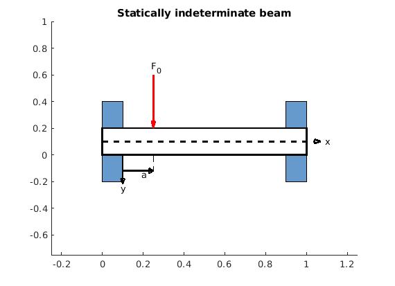
Example 5:
Let us consider a beam of length ℓ rigidly clamped at both ends and loaded by a concentrated force
F0 as shown in figure.
|
|
figure
hold on
rectangle('Position',[0 -0.2 0.1 0.6], 'FaceColor','[0.4 0.6 0.8]')
rectangle('Position',[0.9 -0.2 0.1 0.6], 'FaceColor','[0.4 0.6 0.8]')

w = 0.2 ;
h = 1 ;
x = [0 0 h h] ;
y = [0 w w 0] ;
patch(x, y,'w', 'EdgeColor','k', 'linewidth', 2) ;
title('Statically indeterminate beam') ;
xlim([-0.25 1.25])
ylim([-0.75 1])

% force line

x = [0.25 0.25];
y = [0.6 0.2];
line(x,y,'Color','r','linewidth', 2);
hold on
tri = [0.25 0.26 0.24 0.25; 0.2 0.25 0.25 0.2];
plot(tri(1,:), tri(2,:), 'r', 'linewidth', 1.5)
text(0.24,0.65,'F_0')

% y line

x = [0.1 0.1];
y = [0 -0.2];
line(x, y,'Color','k','linewidth', 2);
hold on
tri = [0.1 0.09 0.11 0.1; -0.22 -0.18 -0.18 -0.22];
plot(tri(1,:), tri(2,:), 'k', 'linewidth', 1.5)
text(0.09, -0.25, 'y')

% a line

x = [0.1 0.25];
y = [-0.12 -0.12];
line(x, y,'Color','k','linewidth', 2);
hold on
tri = [0.25 0.23 0.23 0.25;-0.12 -0.10 -0.14 -0.12];
plot(tri(1,:), tri(2,:), 'k', 'linewidth', 1.5)
text(0.19, -0.15, 'a')

x = [0.25 0.25];
y = [0 -0.12];
line(x, y, 'Color','k','linewidth', 1, 'LineStyle','--');

% x line

x = [0 1.04];
y = [0.1 0.1];
line(x, y,'Color','k','linewidth', 2, 'LineStyle','--');
hold on
tri = [1.07 1.04 1.04 1.07; 0.1 0.085 0.115 0.1];
plot(tri(1,:), tri(2,:), 'k', 'linewidth', 2)
text(1.09, 0.1, 'x')
|
|
Statically interdeterminate beam.
|
|
matlab code
|
The problem is modeled by the
Euler–Bernoulli beam equation
\[
EI\,\frac{{\text d}^4 y}{{\text d}x^4} = F_0 \delta (x-a) , \qquad 0 < x < \ell ,
\tag{4.1}
\]
where
E is the elastic modulus and
I is the second moment of area of the beam's cross-section. Note that
I must be calculated with respect to the axis that passes through the centroid of the cross-section and which is perpendicular to the applied loading.
This equation, describing the deflection of a uniform, static beam, is used widely in engineering practice.
Also, we need to add the boundary conditions for a clamped beam of length ℓ (fixed at
x = 0 and
x = ℓ):
\[
y(0) = 0, \quad y' (0) = 0 \qquad\mbox{and} \qquad y(\ell ) =0, \quad y' (\ell ) = 0 .
\tag{4.2}
\]
Application of the Laplace transform with respect to variable
x yields
\[
\lambda^4 y^L - y'''(0) - \lambda\,y'' (0) - \lambda^2 y' (0) - \lambda^3 y(0) = \frac{F_0}{EI}\, e^{-a\lambda}
\]
Using boundary conditions (4.2) at
x = 0, we obtain the formula for the Laplace transformation of
y(
t):
\[
y^L (\lambda ) = {\cal L} \left[\, y(x)\,\right] = \frac{F_0}{EI}\,\frac{1}{\lambda^4}\, e^{-a\lambda} + \frac{y''' (0)}{\lambda^4} + \frac{y'' (0)}{\lambda^3} .
\tag{4.3}
\]
We denote the unknown derivatives at the origin by
c3 and
c2. Upon application of the inverse Laplace transform, we get
syms t s
ilaplace(1/s^4, s, t)
ilaplace(1/s^3, s, t)
>> ans =
t^3/6
>> ans =
t^2/2
\[
y(x) = \frac{(x-a)^3}{6}\,\frac{F_0}{EI}\,H(x-a) + \frac{x^3}{6}\,c_3 H(x) + \frac{x^2}{2}\,c_2 H(x) ,
\tag{4.4}
\]
where the constants
c3 and
c2 can be determined from the boundary conditions (4.2) at
x = ℓ:
\[
y (\ell ) = \frac{(\ell -a)^3}{6}\, \frac{F_0}{EI} + \frac{\ell^2}{2} \,c_2 + \frac{\ell^3}{6} \, c_3 =0, \qquad y' (\ell ) = \frac{(\ell -a)^2}{2}\, \frac{F_0}{EI} + \ell\,c_2 + \frac{\ell^2}{2}\, c_3 = 0 .
\]
Solving this system of linear equations, we determine
syms l a s t K c2 c3 x
eqn1 = (l - a)^3/6*K + l^3/6*c3 + l^2/2*c2 == 0,
eqn2 = (l - a)^2 /2*K + l*c2 + l^2/2*c3 == 0
[X,Y] = equationsToMatrix([eqn1, eqn2], [c2, c3]);
D = linsolve(X,Y)
simplify(D/K)
>> ans =
(a*(a - l)^2)/l^2
-((a - l)^2*(2*a + l))/l^3
\[
c_2 = \frac{1}{\ell^2}\,\frac{F_0}{EI} \left( a - \ell \right)^2 a , \qquad c_3 = -\frac{1}{\ell^3} \cdot \frac{F_0}{EI} \left( a - \ell \right)^2 \left( 2a + \ell \right) .
\tag{4.5}
\]
The deflection of the beam now is expressed as
\[
y(x) = \frac{F_0}{EI} \left[ \frac{(x-a)^3}{6}\, H(x-a) - \frac{x^3}{6\ell^3} \left( a - \ell \right)^2 \left( 2a + \ell \right) + \frac{x^2}{2\ell^2}\,a \left( a - \ell \right)^2 \right]
\tag{4.6}
\]
Upon introducing the dimensionless variables
\[
\xi = \frac{x}{\ell} , \qquad \alpha = \frac{a}{\ell} ,
\]
the solution becomes
\[
\frac{EI}{F_0 \ell^3}\, y(\xi ) = \frac{1}{6} \left( \xi - \alpha \right)^3 H(\xi - \alpha ) + \left( 1 - \alpha \right)^2 \left[ \frac{\xi^2}{2}\,\alpha - \frac{\xi^3}{6} \left( 1 + 2\alpha \right)\right] .
\tag{4.7}
\]
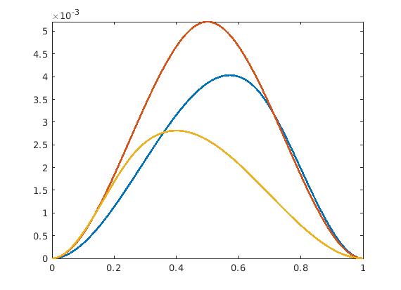
|
|
We plot the deflection curve (4.7) of a beam clamped at both ends in dimensionless coordinated for α = ½, ⅔, and ¼. These graphs show that the maximum deflection occurs when load is applied at the center.
syms l a s t K c2 c3
A = 2/3;
f(x) = (x - A)^3 * heaviside(x - A)/6 + (1 - A)^2 *(x^2 *A/2 - x^3*(1 + 2*A)/6);
fplot(f, [0 1], 'linewidth', 2)
hold on

A = 1/2;
f(x) = (x - A)^3 * heaviside(x - A)/6 + (1 - A)^2 *(x^2 *A/2 - x^3*(1 + 2*A)/6);
fplot(f, [0 1], 'linewidth', 2)

A = 1/4;
f(x) = (x - A)^3 * heaviside(x - A)/6 + (1 - A)^2 *(x^2 *A/2 - x^3*(1 + 2*A)/6);
fplot(f, [0 1], 'linewidth', 2)
|
|
Deflection curve (4.7) of a beam clamped at both ends.
|
|
matlab code
|
■