In this section we develop in detail two bracketing methods for finding a zero/null of a real and continuous function
f(
x). All bracketing methods always converge, whereas open
methods (discussed in the next section) may sometimes diverge. We must start with an initial interval [𝑎,
b], where
f(𝑎) and
f(
b) have opposite signs. Since the graph
y =
f(
x) of a continuous function is unbroken, it will cross the abscissa at a zero
x = α that lies somewhere within the interval [𝑎,
b]. One of the ways to test a numerical method for solving the equation
\( f(x) =0 \) is to check its performance on a polynomial whose roots are known. It is a custom to use some famous polynomials such as
Chebyshev,
Legendre or the
Wilkinson polynomials:
\[
w_n (x) = \prod_{k=1}^n (x-k) = (x-1) (x-2) \cdots (x-n)
\]
that have the roots
\( \{ 1, 2, \ldots , n \} , \) but provide surprisingly tough numerical root-finding problems. For example,
\[
w_9 (x) = x^9 - 45 x^8 + 870 x^7 - 9450 x^6 +
63273 x^5 - 269325 x^4 + 723680 x^3 - 1172700 x^2 + 1026576 x -362880 .
\]
The Bisection Method of Bolzano
Let f be a real single-valued function of a real variable. If
f(α) = 0, then α is said to be a zero of f or null or, equivalently, a root of
the equation f(x) = 0. It is customary to say that
α is a root or zero of an algebraic polynomial f, but just a zero if f is not a polynomial. In this subsection, we discuss an algorithm for finding a root of a function, called the bisection method.
The bisection method is a very simple and
robust algorithm, but it is also relatively slow. The method was invented by the Bohemian mathematician, logician,
philosopher, theologian and Catholic priest of Italian extraction Bernard Bolzano (1781--1848), who spent all his life in Prague (Kingdom of Bohemia, now Czech republic). Most of Bolzano's works remained in manuscript and did not become noticed and therefore did not influence the development of the subject. Many of his works were not published until 1862 or later.
Assume that a continuous function
f(
x) on a given interval [𝑎,
b] satisfies
\[
f(a)\,f(b) < 0.
\]
According to the intermediate value theorem, the function
f(
x) must have at least one root in [𝑎,
b]. Usually [𝑎,
b] is chosen to contain only one root α; but the following algorithm for the bisection method will always converge to some root α in [𝑎,
b].
The bisection method requires two initial guesses 𝑎 = x0 and b = x1 satisfying the bracket condition
f(x0)·f(x1) < 0. As the values of f(x0) and
f(x1) are on opposite sides of the x-axis y = 0, the solution α at which f(α) = 0 must reside somewhere in between of these two guesses, i.e., x0 < α < x1. While any point between the two endpoints can be chosen for the next iteration, we want to avoid the worst possible case in which the solution always happens to be in the larger of the two sections.
The bisection method suggests choosing the middle point in the interval [𝑎, b] as the next approximation to the root α.
The decision step for this process of interval halving is first to choose the midpoint \( c= (a+b)/2 = \left( x_0 + x_1 \right) /2 \) and then to analyze the three possibilities that might arise:
|
Algorithm
|
Bisection (f, 𝑎, b, root, ϵ)
|
|
|
-
Define c:= (𝑎 + b)/2.
- If b - c ≤ ϵ, then accept root:= c, and exit.
- If sign f(b) sign f(c) ≤ 0 (so f(b) and f(c) have opposite signs), then 𝑎:= c; otherwise b:= c.
- Return to step 1.
|

|
|
plot = Plot[1*x^2, {x, 0, 1}, AspectRatio -> 1,
PlotStyle -> {Thickness[0.01], Blue}, Axes -> False,
Epilog -> {PointSize[0.03], Pink, Point[{{0, 0}, {2, 2.8}}]},
PlotRange -> {{-0.5, 1.2}, {-0.2, 1.4}}];
arrow = Graphics[{Arrowheads[0.07], Arrow[{{-0.2, 0.4}, {1.2, 0.4}}]}];
l1 = Graphics[{Thick, Dashed, Line[{{0, 0}, {0, 0.4}}]}];
l2 = Graphics[{Thick, Dashed, Line[{{0.5, 0.25}, {0.5, 0.4}}]}];
l3 = Graphics[{Thick, Dashed, Line[{{0.75, 0.54}, {0.75, 0.4}}]}];
l4 = Graphics[{Thick, Dashed, Line[{{1, 0.4}, {1, 1}}]}];
t1 = Graphics[{Black, Text[Style[Subscript[x, 0], 16], {0, 0.47}]}];
t2 = Graphics[{Black, Text[Style[Subscript[x, 1], 16], {1, 0.35}]}];
t3 = Graphics[{Black, Text[Style[Subscript[x, 2], 16], {0.5, 0.47}]}];
t4 = Graphics[{Black,
Text[Style[Subscript[x, 3], 16], {0.75, 0.35}]}];
t5 = Graphics[{Black, Text[Style[\[Alpha], 16], {0.6, 0.45}]}];
t8 = Graphics[{Black, Text[Style["f(b)", {1.08, 1}]]}];
t9 = Graphics[{Black, Text[Style["f(x)", Bold, 16], {0.5, 0.7}]}];
Show[arrow, plot, l1, l2, l3, l4, t1, t2, t3, t4, t5, t8, t9,
Epilog -> {PointSize[0.02], Purple,
Point[{{0, 0}, {0, 0.4}, {0.5, 0.4}, {0.5, 0.25}, {0.75,
0.555}, {0.75, 0.4}, {1, 0.4}, {1, 1}}]}]
|
|
Bisection iteration.
|
|
Mathematica code
|
If either of the products
\( f(a)\,f(c) \quad\mbox{or} \quad f(c)\,f(b) \) is negative, we have found an interval half as wide as the original interval that contains the root, and we are “squeezing down on it.” To continue the process, relabel the new smaller interval [𝑎,
b] and repeat the process until
the interval is as small as desired. Since the bisection process involves sequences of
nested intervals and their midpoints, we will denote by
\( [a_n , b_n ] \) the subinterval obtained on the
n-th stage of the bisection algorithm. Therefore,
\( [a_0 , b_0 ] \) is just the starting original interval [𝑎,
b]. Its midpoint we denote by
\( c_0 = (a+b)/2 . \) The next interval
\( [a_1 , b_1 ] \) has one of the ends
c0 and the interval is half as wide as the starting one, [𝑎,
b].
After arriving at the n-th interval \( [a_n , b_n ] , \) which brackets r and has midpoint cn, the new interval \( [a_{n+1} , b_{n+1} ] \) is constructed, which also brackets r and is half as wide as \( [a_n , b_n ] . \) So
\[
\left[ a_{n+1} , b_{n+1} \right] = \left[ a_n , c_n \right] \qquad\mbox{or} \qquad \left[ a_{n+1} , b_{n+1} \right] = \left[ c_n , b_n \right] \quad\mbox{for all $n$}.
\]
Theorem (Bolzano): Suppose that
f is a continuous function on the closed interval [𝑎,
b] and that there exists a number α from this interval such that
f(α) = 0. If
f(𝑎) and
f(
b) have opposite signs, and
\( \left\{ c_n \right\}_{n\ge 0} \) represents the sequence of midpoints generated by the bisection algorithm, then
\[
\left\vert \alpha - c_n \right\vert \le \frac{b-a}{2^{n+1}} , \qquad\mbox{for } = 0,1,2,\ldots .
\]
The convergence of the midpoints to the root α is linear (of order 1) and the rate of convergence is one half:
\( \left\vert \alpha - c_{n+1} \right\vert \le ½ \left\vert \alpha - c_n \right\vert . \) ⧫
Although bisection is generally slower than
other methods, the neatness of the procedure (its error analysis, in particular) is a
positive feature that makes bisection attractive. This method is often used in the
built-in root-finding routine of programmable calculators.
One disadvantage of bisection is that it cannot be used to find roots when the
function is tangent to the abscissa and does not pass through it.
function [ zero , res , niter ]= bisection ( fun ,a ,b , tol ,...
nmax , varargin )
% BISECTION Finds function zeros .
% ZERO = BISECTION ( FUN ,A ,B , TOL , NMAX ) tries to find a zero
% ZERO of the continuous function FUN in the interval
% [A , B ] using the bisection method . FUN accepts real
% scalar input x and returns a real scalar value . If
% the search fails an error message is displayed .
% FUN can be either an inline function or an anonymous
% function or it can be defined by an external m - file .
% ZERO = BISECTION ( FUN ,A ,B , TOL , NMAX , P1 , P2 ,...) passes
% parameters P1 , P2 ,... to the function FUN (X , P1 , P2 ,...)
% [ ZERO , RES , NITER ]= BISECTION ( FUN ,...) returns the value
% of the residual in ZERO and the iteration number at
% which ZERO was computed .
x = [a , ( a + b )*0.5 , b ];
fx = feval ( fun ,x , varargin {:});
if fx (1)* fx (3) > 0
error ([ ’ The sign of the function at the ’ ,...
’ endpoints of the interval must be different \ n ’ ]);
elseif fx (1) == 0
zero = a ; res = 0; niter = 0; return
elseif fx (3) == 0
zero = b ; res = 0; niter = 0; return
end
niter = 0;
I = ( b - a )*0.5;
while I >= tol & niter < nmax
niter = niter + 1;
if fx (1)* fx (2) < 0
x (3) = x (2);
x (2) = x (1)+( x (3) - x (1))*0.5;
fx = feval ( fun ,x , varargin {:});
I = ( x (3) - x (1))*0.5;
elseif fx (2)* fx (3) < 0
x (1) = x (2);
x (2) = x (1)+( x (3) - x (1))*0.5;
fx = feval ( fun ,x , varargin {:});
I = ( x (3) - x (1))*0.5;
else
x (2) = x ( find ( fx ==0)); I = 0;
end
end
if ( niter == nmax & I > tol )
fprintf ([ ’ Bisection stopped without converging ’ ,...
’ to the desired tolerance because the \ n ’ ,...
’ maximum number of iterations was reached \ n ’ ]);
end
zero = x (2);
x = x (2);
res = feval ( fun ,x , varargin {:});
return
Pseudocode for Bisection Method:
input a,v,eps

external f

fa = f(a)

fb = f(b)

if f(a)*f(b) > 0 then stop

n = fix((log(b-a) - log(eps))/log(2)) + 1

for i=1 to n do

	c = a+0.5*(b-a)

	fc = f(c)

	if fa*fc < 0 then

		b = c

		fb = fc

	else

		if fa*fc > 0 then

		a = c

		fa = fc

	else

		alpha = c

		return

	endif

endif

endfor
Example 1:
Consider qubic equation
\[
x^3 + x^2 -3\,x -3 = 0,
\]
on the interval [0,2]. We find its root on this interval with an error tolerance of 10
-6. It is always a good idea to plot the function

|
|
Plot[x^3 + x^2 - 3*x - 3, {x, -2.4, 2}, PlotStyle -> Thick,
PlotLabel -> Style["x^3 + x^2 - 3x-3", FontSize -> 16],
Background -> LightBlue]
|
|
Graph of the cubic function.
|
|
Mathematica code
|
The bisection method is a bracketing type root finding method in which the interval
is always divided in half. If a function changes sign over an interval, the function
value at the midpoint is evaluated. The location of the root is then determined as
lying within the subinterval where the sign change occurs. The subinterval then
becomes the interval for the next iteration. The process is repeated until the root is
known to the required precision.
Now we ask matlab do 20 iterations and present the output in table format:
clearvars;
syms x
y = x^3+x^2-3*x-3;
ezplot(y) % we start out by plotting the function
xlim([-3,3])
ylim([-5,3])

%% Part 2:
% We iterate the function below and place the results in table form
clearvars;
f = @(x) x^3+x^2-3*x-3;
root =bisection(f,1,2,1e-10);
function c = bisection(f,a,b,tol)%f=@(x)x^2-3; a=0; b=2; (ensure change of sign between a and b) error=1e-4
c=(a+b)/2;
while abs(f(c))>tol
    if f(c)<0&&f(a)<0
        a=c;
    else
        b=c;
    end
    c=(a+b)/2;
end
end
clearvars;
a = 1;
b = 2;
E = 1e-10;
N = 10;
f = @(x) x^3+x^2-3*x-3;
format long
for i = 1:N
    c =(a+b)/2;
    T = table(N,a,b,c,f(c));
    T(N:5,:)
    disp(T);
    if f(c) * f(a) > 0
        a = c;
    else
        b = c;
    end
%     if (abs(b-a) / 2^N) <= E || f(c) == 0

%         break
%     end
end
0,       2,       1.,      -3.,        3.,        -4.
1.,      2,       1.5,     -4.,        3.,        -1.875
1.5,     2,       1.75,    -1.875,     3.,         0.171875
1.625,   1.75,    1.6875,  -0.943359,  0.171875}  -0.943359
1.625,   1.75,    1.6875,  -0.943359,  0.171875,   -0.409424
1.6875,  1.75,    1.71875, -0.409424,  0.171875,   -0.124786
1.71875, 1.75,    1.73438, -0.124786,  0.171875,    0.0220299
1.71875, 1.73438, 1.72656, -0.124786,  0.0220299,  -0.0517554
1.72656, 1.73438, 1.73047, -0.0517554, 0.0220299,  -0.0149572
1.73047, 1.73438, 1.73242, -0.0149572, 0.0220299,   0.00351267
1.73047, 1.73242, 1.73145, -0.0149572, 0.00351267, -0.0057282
Finally, we check our answer with
Mathematica:
FindRoot[-3 - 3 x + x^2 + x^3 , {x, 1.7}]
{x -> 1.73205}
The root and the function value at the root are computed by the m-file. Figure displays the graph of the polynomial and the location of the root.
Bisection method used in this case (with error tolerance of 10−6) stops at the end of
21th iteration.
Note that the Octave code uses 𝑎 + 0.5(b − 𝑎) as the basic equation of bisection. The
reason is that for very large values of 𝑎, b, (𝑎 + b)/2 can lead to a computational overflow.
■
Example 2:
Consider the function \( f(x) = e^x\, \cos x - x\, \sin x \) that has three nulls on the interval [0,10], and Mathematica confirms
f[x_] = Exp[x]*Cos[x] - x*Sin[x]
FindRoot[f[x] == 0, {x, 1.5}]
Out[2]= {x -> 1.22539}
FindRoot[f[x] == 0, {x, 4.5}]
Out[3]= {x -> 4.6686}
FindRoot[f[x] == 0, {x, 8}]
Out[4]= {x -> 7.85092}
|
Graph of the function \( f(x) = e^x\, \cos x - x\, \sin x . \)
|
|
First, we plot the given function in a neighborhood of the origin.
f[x_] = Exp[x]*Cos[x] - x*Sin[x]
a = -1.0;
b = 2.0;
Bisection[a, b, 30];
Plot[f[x], {x, -1.05, 2.05}, PlotRange -> {{-1.05, 2.05}, {-5, 1.5}},
PlotStyle -> {Magenta,Thick}]
|
We bracket the first root by the interval [0,3] because
\( f(0)\, f(3) \approx -20.3079 . \) Dividing it in half, we choose the middle point
\( c_0 =1.5, \) with
\( f(0)\, f(1.5) \approx -1.17922 . \) Since the latter product is negative, our next interval will be
\( [a_1 , b_1 ] = [0 , 1.5] . \) Its middle point is
\( c_1 = 0.75 . \) Since
\( f(0.75)\, f(1.5) \approx -1.22374 , \) we choose
\( [a_2 , b_2 ] = [0.75 , 1.5] . \) Its middle point is
\( c_2 = 1.125 . \) Since
\( f(1.125)\, f(1.5) \approx -0.369174 , \) we choose
\( [a_3 , b_3 ] = [1.125 , 1.5] . \) Again, we halve it to obtain the midpoint
\( c_3 = 1.3125 . \) Since
\( f(1.125)\, f(1.3125) \approx -0.100152 , \) we choose
\( [a_4 , b_4 ] = [1.125 , 1.3125] . \) We can continue this process, but we see that convergence to the zero
r = 1.22539 of the function
f is slow: only fifth iteration gave us the first correct decimal place after the period.
Now we show step by step how it works using Mathematica. First we plot the function to roughly identify the roots.
f[x_] := Exp[x]*Cos[x] - x*Sin[x]
Plot[f[x], {x, 0, 8}, PlotStyle -> {Thick, Blue}]
Graph of the function \( f(x) = e^x\, \cos x - x\, \sin x . \)
Then we define the range of x you want to see the function
xa = 0; xb = 3;
curve = Plot[f[x], {x, xa, xb},
PlotLabel -> "Entered function on given interval",
LabelStyle -> {FontSize -> 11}];
We break the guess interval [0,3] into 10 uniform parts and calculate the values of the given function at each end point of these subintervals.
maxi = f[xa]; mini = f[xb];
step = (xb - xa)/10;
x[0] = xa;
Do[ x[i] = x[i - 1] + step; If[f[x[i]] > maxi, maxi = f[x[i]];
If[f[x[i]] < mini, mini = f[x[i]]]];
Print["i= ", i, ", x[i]= ", x[i], ", f[x[i]]= ", N[f[x[i]]]];
, {i, 1, 10}]
So we see that the first root is within the interval [6/5, 3/2].
xa = 6/5; xb = 3/2; maxi = f[xa]; mini = f[xb];
Show[Graphics[Line[{{xa, maxi}, {xa, mini}}]], curve,
Graphics[Line[{{xb, maxi}, {xb, mini}}]], Axes -> True,
PlotLabel ->
"Entered function on given interval with upper and lower guesses",
LabelStyle -> {FontSize -> 11},
PlotRange -> {{0.25, 2}, {-1.3, 0.6}}]
Now we check whether the center of this interval is closer to the root:
xc = (xa + xb)/2;
If[f[xa]*f[xc] <= 0, xb = xc]
27/20
Therefore, we find that the root is within the interval [6/5,27/20] or [1.2 , 1.35]. Finding the value of the function at the lower and upper guesses and the estimated root:
N[f[xa]]
N[f[xb]]
0.0846232
-0.472425
We plot the root bracketing with two iterations:
Show[Graphics[Line[{{xa, maxi}, {xa, mini/2}}]], curve,
Graphics[Line[{{3/2, maxi}, {3/2, mini/2}}]],
Graphics[Line[{{27/20, maxi}, {27/20, mini/2}}]], Axes -> True,
PlotLabel ->
"Entered function on given interval with upper and lower guesses
and estimated root", LabelStyle -> {FontSize -> 10},
PlotRange -> {{0.5, 1.8}, {-0.6, 0.2}}]
Now we do the third iteration:
xc = (xa + xb)/2
N[xc]
51/40
1.275
We check the interval between which the root lies.
xc = (xa + xb)/2;
If[f[xa]*f[xc] <= 0, xb = xc]
Show[Graphics[Line[{{xa, maxi}, {xa, mini/4}}]], curve,
Graphics[Line[{{3/2, maxi}, {3/2, mini/4}}]],
Graphics[Line[{{51/40, maxi}, {51/40, mini/4}}]],
Graphics[Line[{{27/20, maxi}, {27/20, mini/4}}]], Axes -> True,
PlotLabel -> "Function on given interval with estimated root",
LabelStyle -> {FontSize -> 10},
PlotRange -> {{0.8, 1.7}, {-0.35, 0.1}}]
Here the bisection method algorithm is applied to generate the values of the roots, true error, absolute relative true error, approximate error, absolute relative approximate error, and the number of significant digits at least correct in the estimated root as a function of number of iterations.
nmaximum = 30; (* Maximum number of iterations *)
For[i = 1; xu = xb; xl = xa, i <= nmaximum, i++, xr[i] = (xu + xl)/2;
If[f[xr[i]]*f[xu] <= 0, xl = xr[i], xu = xr[i]]]
Absolute true error:
Array[Et, nmaximum]; (* Array of absolute error *)
s = FindRoot[Exp[x]*Cos[x] - x*Sin[x] == 0, {x, 1.2}]
xactual = Evaluate[x /. s]
For[i = 1, i <= nmaximum, i++, Et[i] = Abs[xactual - xr[i]]]
Absolute relative true error:
Array[et, nmaximum]; (* Array of absolute relative errors *)
For[i = 1, i <= nmaximum,
i++, et[i] = Abs[Et[i]/xactual*100]]
Absolute approximate error:
Array[Ea, nmaximum]; (* Array of absolute approximate errors *)
For[i = 1, i <= nmaximum, i++,
If[i <= 1, Ea[i] = 0, Ea[i] = Abs[xr[i] - xr[i - 1]]]]
Absolute relative approximate error:
Array[ea, nmaximum]; (* Array of absolute relative errors *)
For[i = 1, i <= nmaximum, i++,
If[i <= 1, ea[i] = 0, ea[i] = Abs[Ea[i]/xr[i]*100]]]
Significant digits at least correct
Array[sigdig, nmaximum]; (* Array of correct digits *)
For[i = 1, i <= nmaximum, i++,
If[(ea[i] >= 5) || (i <= 1), sigdig[i] = 0,
sigdig[i] = Floor[(2 - Log[10, Abs[ea[i]/0.5]])]]]
Graphs
xrplot = Table[xr[i], {i, 1, nmaximum}];
ListPlot[xrplot, Joined -> True, PlotRange -> All,
AxesOrigin -> {1, Min[xrplot]},
PlotLabel -> "Estimated root as a function of number of iterations"]
Etplot = Table[Et[i], {i, 1, nmaximum}];
ListPlot[Etplot, Joined -> True, PlotRange -> All,
AxesOrigin -> {1, Min[Etplot]},
PlotLabel ->
"Absolute true error as a function of number of iterations"]
etplot = Table[et[i], {i, 1, nmaximum}];
ListPlot[etplot, Joined -> True, PlotRange -> All,
AxesOrigin -> {1, Min[etplot]},
PlotLabel ->
"Absolute relative true error as a function of number of iterations"]
Eaplot = Table[Ea[i], {i, 1, nmaximum}];
ListPlot[Eaplot, Joined -> True, PlotRange -> All,
AxesOrigin -> {1, Min[Eaplot]},
PlotLabel ->
"Absolute approximate error as a function of number of iterations"]
eaplot = Table[ea[i], {i, 1, nmaximum}];
ListPlot[eaplot, Joined -> True, PlotRange -> All,
AxesOrigin -> {1, Min[eaplot]},
PlotLabel ->
"Absolute relative approximate error as a function of number of iterations"]
sigdigplot = Table[sigdig[i], {i, 1, nmaximum}];
BarChart[sigdigplot]
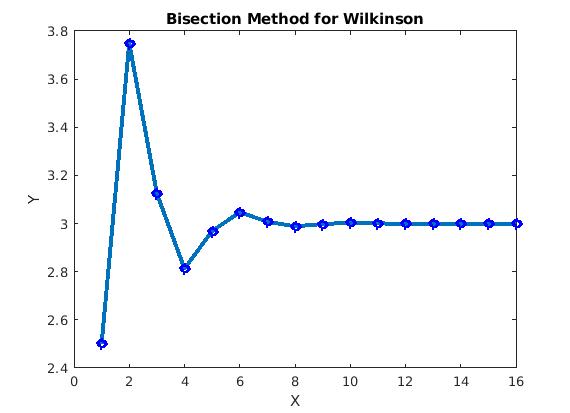
Example 3:
We consider the Wilkinson polynomial:
\[
-5040 + 13068*x - 13132*x^2 + 6769*x^3 - 1960*x^4 + 322*x^5 - 28*x^6 + x^7
\]
clear all;
close all;
clc;
format long e
a = 0;
b = 5;
n = 1e-4;
N = ceil(log((b - a) / n) / log(2));
f = @(x) -5040 + 13068*x - 13132*x^2 + 6769*x^3 - 1960*x^4 + 322*x^5 - 28*x^6 + x^7;
iter = 1;
mData = [];
T = table('Size', [N, 5], ...
    'VariableTypes', {'double', 'double', 'double', 'double', 'double'}, ...
    'VariableNames', {'N', 'a', 'b', 'c', 'fc'});

% tol = this eq & set error 10^-3
%n = fix((log(b-a ) - log(eps))/log(2)) + 1
while (abs(a-b)>n)
fa = f(a);
fb = f(b);
c = a + 0.5*(b - a);
fc = f(c);
T(iter, :) = {iter, a, b, c, f(c)};
    if (fa*fc < 0)
    b = c
    fb = fc
    else
    a = c;
    fa = fc;
    alpha = c;
    end
    mData([iter]) = c; % save data to array
    iter = iter + 1 ;
    fprintf('%d \t %f \f \t %f \t %f \t %f\n',iter,a,b, abs(a-b),n);
end

l = plot(mData) % plot data

xlabel('X');
ylabel('Y');
title('Bisection Method for Wilkinson');
l.LineWidth = 3;
l.Marker = 'o';
l.MarkerEdgeColor = 'b';

%%creates a column vector that shows the different approximations for each
%%iteration.
mData'

disp(T)
We present some scripts for the application of the bisection method. First, we type in a subroutine for halving the interval.
shrinkInterval[func_, {a_?NumericQ, b_?NumericQ}] /; a < b :=
Module[{interval}, interval = {a, (a + b)/2, b};
Last@Flatten[
Select[Thread@(Partition[#, 2,
1] & /@ {Sign /@ (func /@ interval), interval}),
Times @@ (First@#) < 0 &], 1]]
Then we apply this subroutine to perform bisection algorithm with tolerance ξ.
biSection[func_, {a0_?NumericQ, b0_?NumericQ}, \[Xi]_?NumericQ] :=
NestWhile[shrinkInterval[func, #] &, {a0, b0},
Abs@(Subtract @@ #) > \[Xi] &]
Here is a demonstration of how to use the code above to find the null of the function
\( f(x) = e^x\, \cos x - x\, \sin x \) based on the bisection method:
biSection[Exp[#]*Cos[#] - #*Sin[#] &, {0, 1.5`20}, .5*10^-15]
Out[3]= {1.2253937841236203221, 1.2253937841236206552}
Another code:
f[x_] = Exp[x]*Cos[x] - x*Sin[x]
a[1] = 0;
b[1] = 3;
Do[p[n] = N[1/2 (a[n] + b[n])];
If[N[f[b[n]] f[p[n]]] < 0, a[n + 1] = p[n]; b[n + 1] = b[n],
a[n + 1] = a[n]; b[n + 1] = p[n]], {n, 1, 20}]
TableForm[
Table[{a[n], b[n], p[n], N[f[a[n]]], N[f[b[n]]], N[f[p[n]]]}, {n, 1,
20}]]
Another code:
Clear["`*"];
f[x_] = Exp[x]*Cos[x] - x*Sin[x]
Plot[f[x], {x, 0, 9}];
a = Input["Enter a"];
b = Input["Enter b"];
tol = Input["Enter tolerance"];
n = Input["Enter total iteration"];
If[f[a]*f[b] > 0, {Print["No solution exists"] Exit[]}];
Print[" n a b c f(c)"];
Do[{c = (a + b)/2;
If[f[a]*f[c] > 0, a = c, b = c],
Print[PaddedForm[i, 5], PaddedForm[N[a], {10, 6}],
PaddedForm[N[b], {10, 6}], PaddedForm[N[c], {10, 6}],
PaddedForm[N[f[c]], {10, 6}]]
If[
Abs[a - b] < tol, {Print["The solution is: ", c] Exit[]}]}, {i,
1, n}];
Print["The maximum iteration failed"];
The poor convergence of the bisection method as well as its poor adaptability to higher dimensions (i.e., systems of two or more non-linear equations) motivate the use of better techniques. Another popular algorithm is the method of false position or the regula falsi method. A better approach is obtained if we find the point c on the abscissa where the secant line crosses it. To determine the value of c, we write down two versions of the slope m f the line that connects the points \( (a, f(a)) \quad\mbox{and} \quad (b, f(b)) : \)
\[
m = \frac{f(b) - f(a)}{b-a} = \frac{0-f(b)}{c-b} ,
\]
where points
\( (a, f(a)) ,\quad (b, f(b)) , \quad\mbox{and} \quad (c,0) \) were used. Solving for
c, we get
\[
c = b - \frac{f(b) \left( b-a \right)}{f(b)-f(a)} .
\]
The three possibilities are the same as before:
- If f(a) and f(c) have opposite signs, a zero lies in [a,c] .
- If f(b) and f(c) have opposite signs, a zero lies in [c,b] .
- If \( f(c) =0 , \) then the zero is c.

|
|
plot = Plot[1*x^2, {x, 0, 1}, AspectRatio -> 1,
PlotStyle -> {Thickness[0.01], Blue}, Axes -> False,
Epilog -> {PointSize[0.03], Pink, Point[{{0, 0}, {1, 1}}]},
PlotRange -> {{-0.2, 1.2}, {-0.2, 1.4}}];
line = Graphics[{Thick, Red, Line[{{0, 0}, {1, 1}}]}];
arrow = Graphics[{Arrowheads[0.07], Arrow[{{-0.2, 0.3}, {1.2, 0.3}}]}];
l1 = Graphics[{Thick, Dashed, Line[{{0, -0.1}, {0, 0.3}}]}];
l3 = Graphics[{Thick, Dashed, Line[{{1, 0.3}, {1, 1}}]}];
t1 = Graphics[{Black, Text[Style["a", 16], {0, 0.36}]}];
t3 = Graphics[{Black, Text[Style["f(a)", 16], {-0.08, 0.0}]}];
t4 = Graphics[{Black, Text[Style[\[Alpha], 16], {0.55, 0.23}]}];
t5 = Graphics[{Black, Text[Style["c", 16], {0.3, 0.36}]}];
t6 = Graphics[{Black, Text[Style["b", 16], {1, 0.23}]}];
t8 = Graphics[{Black, Text[Style["f(b)", {1.08, 1}]]}];
t9 = Graphics[{Black, Text[Style["f(x)", Bold, 16], {0.87, 0.56}]}];
Show[arrow, plot, line, l1, l3, t1, t3, t4, t5, t6, t8, t9,
Epilog -> {PointSize[0.02], Purple,
Point[{{0, 0}, {0, 0.3}, {0.3, 0.3}, {0.55, 0.3}, {1, 1}, {1,
0.3}}]}]
|
|
Regula Falsi.
|
|
Mathematica code
|
The decision process is the same as in bisection method and we generate a sequence of intervals
\( \left\{ [a_n , b_n ]\right\} \) each of which brackets the null. At each step the approximation of the zero
r is
\[
c_n = b_n - \frac{f(b_n ) \left( b_n -a_n \right)}{f(b_n )-f(a_n )} , \qquad n=0,1,2, \ldots .
\]
This method is called regular falsi (false position method) and it was known to ancient Babylonian mathematicians. It has also linear rate of convergence of
the sequence
\( \left\{ c_n \right\}_{n\ge 0} \) to the null
r of the function
f. But beware: although the integral
width
\( b_n - a_n \) is getting smaller, it is possible that it may not go to zero. If the graph of
\( y= f(x) \) is concave near
(r,0), one of the endpoints becomes fixed and the other does not march into the solution.
Example 4:
We reconsider the function \( f(x) = e^x\, \cos x - x\, \sin x \) on
interval [0,3]. From the previous example, we know that f has the null r = 1.22539. We ask matlab
for help:
clear all;
close all;
clc;
format long
a = 0;
b = 5;
n = 1e-4;
N = 100
%fix(log((b - a) / n) / log(2));
f = @(x) exp(x)*cos(x) - x*sin(x);
iter = 1;
mData = [];
T = table('Size', [N, 5], ...
    'VariableTypes', {'double', 'double', 'double', 'double', 'double'}, ...
    'VariableNames', {'N', 'a', 'b', 'c', 'fc'});
% tol = this eq & set error 10^-3
%n = fix((log(b-a ) - log(eps))/log(2)) + 1
for i = 1:N
fa = f(a);
fb = f(b);
c = b - (f(b)*((a-b))/(f(a)-f(b)));
fc = f(c);
T(iter, :) = {iter, a, b, c, f(c)};
    if (fa*fc < 0)
    b = c
    fb = fc
    else (fa*fc > 0)
    a = c;
    fa = fc;
  %  alpha = c;
    end
    mData([iter]) = c; % save data to array
    iter = iter + 1 ;
    fprintf('%d \t %f \f \t %f \t %f \t %f\n',iter,a,b, abs(a-b),n);
end
l = plot(mData) % plot data


xlabel('X');
ylabel('Y');
title('False Position Method for f = exp(x)*cos(x)-x*sin(x)');
l.LineWidth = 3;
l.Marker = 'o';
l.MarkerEdgeColor = 'b';

%%creates a column vector that shows the different approximations for each
%%iteration.
mData'

disp(T)
f[x_] = Exp[x]*Cos[x] - x*Sin[x]
a = Input["Enter a"];
b = Input["Enter b"];
tol = Input["Enter tolerance"];
n = Input["Enter total iteration"];
x0 = a;
x1 = b;
If[f[x0]*f[x1] > 0, {Print["There is no root in this interval"],
Exit[]}];
Print[" n x0 x1 x2 f(x2)"];
Do[x2 = x0 - (f[x0]/(f[x1] - f[x0]))*(x1 - x0) // N;
Print[PaddedForm[i, 5], PaddedForm[x0, {12, 6}],
PaddedForm[x1, {12, 6}],
PaddedForm[x2, {12, 6}],
PaddedForm[f[x2], {12, 6}]];
If[Abs[x2 - x1] < tol ||
Abs[x2 - x0] < tol, {Print["The root is: ", x2], Exit[]}];
If[f[x0]*f[x2] > 0, x0 = x2, x1 = x2], {i, 1, n}];
Print["Maximum iteration failed"];
Using the above code, we conclude that after 100 iterations the approximate value is 1.20382, which is far away from the true one.
A powerful variant on false position was proposed in 1979 by C.J.F. Ridders. The idea of the method is to apply the regula falsi to the equation
h(
x) = 0 instead of
f(
x) = 0, where
\( h(x) = f(x)\, e^{mx} \) because both functions,
f and
h, have the same roots. In many cases, multiplication by an exponential function may facilitate determination of the root of
f(
x) because its bracketing could be highlighted. One might expect a faster convergence of this method because of a better approximation of the function
f(
x). However, there is a price to pay: the algorithm is a bit more complex and an additional calculation of the function beyond the bracketing points is required.

|
|
plot = Plot[1*x^2, {x, 0, 1}, AspectRatio -> 1,
PlotStyle -> {Thickness[0.01], Blue}, Axes -> False, PlotRange -> {{-0.2, 1.2}, {-0.2, 1.4}} ]
line = Graphics[{Thick, Red, Line[{{0, -0.1}, {1, 0.8}}]},
Epilog -> {PointSize[0.03], Pink, Point[{{0.5, 0.5}}]}];
arrow = Graphics[{Arrowheads[0.07], Arrow[{{-0.2, 0.3}, {1.2, 0.3}}]}];
l1 = Graphics[{Thick, Dashed, Line[{{0, -0.1}, {0, 0.3}}]}];
l2 = Graphics[{Thick, Dashed, Line[{{0.5, 0.25}, {0.5, 0.35}}]}];
l3 = Graphics[{Thick, Dashed, Line[{{1, 0.3}, {1, 1}}]}];
t1 = Graphics[{Black, Text[Style[Subscript[x, 1], 16], {0, 0.36}]}];
t2 = Graphics[{Black, Text[Style[Subscript[h, 1], 16], {0, -0.16}]}];
t3 = Graphics[[{Black,
Text[Style[Subscript[f, 1], 16], {-0.08, 0.0}]}];
t4 = Graphics[{Black, Text[Style["u", 16], {0.5, 0.17}]}];
t5 = Graphics[{Black,
Text[Style[Subscript[x, 3], 16], {0.44, 0.36}]}];
t6 = Graphics[{Black, Text[Style[Subscript[x, 2], 16], {1, 0.26}]}];
t7 = Graphics[{Black, Text[Style[Subscript[h, 2], 16], {1.08, 0.8}]}];
t8 = Graphics[{Black, Text[Style[Subscript[f, 2], 16], {1.08, 1}]}];
t9 = Graphics[{Black, Text[Style["f(x)", Bold, 16], {0.75, 0.76}]}];
Show[arrow, plot, line, l1, l2, l3, t1, t2, t3, t4, t5, t6, t7, t8,
t9, Epilog -> {PointSize[0.02], Purple,
Point[{{0, -0.1}, {0, 0}, {0, 0.3}, {0.45, 0.3}, {0.5, 0.3}, {1,
0.8}, {1, 1}, {1, 0.3}}]}]
|
|
Ridders’ algorithm.
|
|
Mathematica code
|
When a root is bracketed between x1 and x2, Ridders’ method first evaluates the function h(x) at the midpoin \( u = \left( x_1 + x_2 \right) /2 . \) Then for three equidistance x-values x1, u, and x2, the following requirement for the straight line connecting points (x1, f1) and (x2, f2) is met:
\[
h_2 -2\,h_u + h_1 = 0 ,
\]
where
\[
h_1 = f\left( x_1 \right) e^{m\,x_1} = f_1 e^{m\,x_1} , \qquad h_u = f\left( u \right) e^{m\,u} = f_u e^{m\,u} , \qquad h_2 = f\left( x_2 \right) e^{m\,x_2} = f_1 e^{m\,x_2} .
\]
Let
\( d = \left( x_2 - x_1 \right) /2 = u - x_1 = x_2 - u \) and the bracketing condition
f1·
f2 < 0 holds, then from the requirement condition we derive
\[
f_2 \,e^{2m\,d} - 2\, f_u e^{m\,d} + f_1 = 0 .
\]
Since this is a quadratic equation in
em d, it can be analytically solved to give
\[
e^{m\,d} = \frac{1}{f_2} \left[ f_u - \mbox{sign}\left( f_1 \right) \sqrt{f_u^2 - f_1 f_2} , \right]
\]
where sign(
x) stands for the sign of the function’s argument:
\[
\mbox{sign}\left( x \right) = \begin{cases}
\phantom{-}1, & \ \mbox{ for } \ x > 0, \\
\phantom{-}0, & \ \mbox{ for } \ x = 0, \\
-1, & \ \mbox{ for } \ x < 0 . \end{cases}
\]
Finally, application of the false position method to the points
hu and either
h1 or
h2 (depending which pair brackets the root) yields a new guess for the root,
x3
\[
x_3 = \frac{x_1 + x_2}{2} + \left( u - x_1 \right) \frac{\mbox{sign} \left[ f(x_1 ) - f(x_2 ) \right] f(u )}{\sqrt{f^2 (u ) - f(x_1 )f(x_2 )}} , \qquad\mbox{with} \quad u = \frac{x_1 + x_2}{2} .
\]
This formula has some very nice properties. First,
x3 is guaranteed to lie in the interval
\( \left( x_1 , x_2 \right) , \) so the Ridders’ method never jumps out of its brackets. Second, the convergence of successive applications of the above formula is
quadratic. Since each application of Ridders’ formula requires two function
evaluations, the actual order of the method is
\( \sqrt{2} , \) not 2; but this is still quite
respectably superlinear: the number of significant digits in the answer approximately doubles with each two function evaluations. Third, taking out the function’s “bend” via exponential (that is, ratio) factors, rather than via a polynomial technique (e.g., fitting a parabola), turns out to give an extraordinarily robust algorithm. In both reliability and speed, Ridders’ method is generally competitive with the more highly developed and better established (but more complicated) method of Van Wijngaarden,
Dekker, and Brent, which we discuss next.
|
Algorithm:
|
Ridders’ rule for determination of the root of the equation f(x) = 0
|
|
|
-
Find proper bracketing points x1 and x2 for the root α of the equation f(x) = 0. It is irrelevant which is positive end and which is negative, but the function must have different signs at these points, i.e., f(x1)×f(x2) < 0.
-
Start loop.
-
Find the midpoint \( u = \left( x_2 - x_1 \right) . \)
-
Find a new approximation for the root
\[
x_3 = \frac{x_1 + x_2}{2} + \frac{x_2 - x_1}{2} \cdot \frac{\mbox{sign} \left[ f(x_1 ) - f(x_2 ) \right] f(u )}{\sqrt{f^2 (u ) - f(x_1 )f(x_2 )}} , \qquad\mbox{with} \quad u = \frac{x_1 + x_2}{2} .
\]
-
If x3 satisfies the required precision and the convergence condition is reached, then stop.
-
Rebracket the root, i.e., assign new x1 and x2, using old values:
-
one end of the bracket is x3 and f3 = f(x3);
-
the other is whichever of (x1, x2, u) is closer to x3 and provides the proper bracket.
-
Repeat the loop.
|
Example 5:
Consider the Bessel function of the first kind of order 1/4:
\[
J_{1/4} \left( x \right) = \sum_{k\ge 0} \frac{(-1)^k}{k!\,\Gamma \left( k + \frac{1}{4} + 1 \right)}\left( \frac{x}{2} \right)^{2k+1/4} .
\]

|
|
We plot the Bessel function with the following Mathematica code:
Plot[BesselJ[1/4, x], {x, 0, 10}, PlotStyle -> Thick,
PlotLabel -> Style["Bessel function of order 1/4", FontSize -> 16],
Background -> LightBlue]
|
|
Bessel function of order 1/4.
|
|
Mathematica code
|
Since the Bessel function has a positive value at
x = 2
N[BesselJ[1/4,2]]
0.397811
and a negative value at
x = 4
N[BesselJ[1/4,4]]
-0.374761
we know that one of its roots belongs to the interval [2,4]. So we start with first two approximations
x0 = 2 and
x1 = 4. The middle point is obviously
u = 3. According to Ridders' formula, our next iteration is
\[
x_2 = 3 + 1 \cdot \frac{J_{1/4}(3)}{\sqrt{J_{1/4}^2 (3) - J_{1/4}(0=2) \cdot J_{1/4}(4)}} = 0.090012 .
\]
x2 = 3 + 1*N[BesselJ[1/4, 3]]/Sqrt[BesselJ[1/4, 3]^2 - BesselJ[1/4, 2]*BesselJ[1/4, 4]]
2.74779
The true value of the root is
FindRoot[BesselJ[1/4, x], {x, 3}]
{x -> 2.78089}
■
To roughly estimate the locations of the roots of the equation \( f(x) =0 \) over the interval [a,b], it make sense to make a uniform partition of the interval by sample points \( \left( x_n , y_n = f(x_n )\right) \) and use the following criteria:
\[
\begin{split} (y_{n-1})(y_n ) < 0 \quad \mbox{or} \\
|y_n | < \epsilon \quad\mbox{and} \quad (y_n - y_{n-1})(y_{n+1} - y_n ) < 0. \end{split}
\]
That is, either
\( f(x_{n-1}) \quad\mbox{and} \quad f(x_n ) \) have opposite signs or
\( |f(x_n )| \) is small and slope of the curve
\( y= f(x) \) changes sign near
\( \left( x_n , f(x_n )\right) . \)
■
================================== Example 1 ================
Example 1:
Consider qubic equation
\[
x^3 + x^2 -3\,x -3 = 0,
\]
on the interval [0,2]. We find its root on this interval with an error tolerance of 10
-6.
The reliable, fail-safe portion of zeroin is the bisection algorithm. The idea is to repeatedly cut the interval [a,b]
in half, while continuing to span a sign change. The actual function values are not used, only the signs. Here is the code for bisection by itself.
https://blogs.mathworks.com/cleve/2015/10/12/zeroin-part-1-dekkers-algorithm/
function b = bisect(f,a,b)
   s = '%5.0f %19.15f %19.15f\n';
   fprintf(s,1,a,f(a))
   fprintf(s,2,b,f(b))
   k = 2;
   while abs(b-a) > eps(abs(b))
      x = (a + b)/2;
      if sign(f(x)) == sign(f(b))
         b = x;
      else
         a = x;
      end
      k = k+1;
      fprintf(s,k,x,f(x))
   end
end
Let's see how bisect performs on our test function. The interval [3,4] provides a satisfactory starting interval because IEEE floating point arithmetic generates a properly signed infinity, +Inf, at the pole.
Another code:
k = 0;
while abs(b-a) > eps*abs(b)
   x = (a + b)/2;
   if sign(f(x)) == sign(f(b))
      b = x;
   else
      a = x;
   end
k = k+1;
end
figure(1)
plot(x, y, 'Color', [1 0 0]) %blue line
hold on
plot(x, z, 'Color', [0 1 0]) %green line