MATLAB TUTORIAL for the First Course. Part 4: Second and Higher Order ODEs

Prof. Vladimir A. Dobrushkin

This tutorial contains many Matlab scripts.
You, as the user, are free to use all codes for your needs, and have the right to distribute this tutorial and refer to this tutorial as long as this tutorial is accredited appropriately. Any comments and/or contributions for this tutorial are welcome; you can send your remarks to

Email Vladimir Dobrushkin

Fundamental Set of Solutions


I. The build-in matlab function ode45

matlab can be used to solve numerically second and higher order ordinary differential equations subject to some initial conditions by transfering the problem into equivalent 2 x 2 system of ordinary differential equations of first order. A function for numerical solution of such systems is, for example, \( \texttt{ode45} \) . Documentation for \( \texttt{ode45} \) states the standard usage format. One can get more advanced information by including more input/output parameters, but we start with a simplest case.

[Tout, Yout] = ode45(ODEFUN,TSPAN,Y0)

Deciphering this definition, we see that \( \texttt{ode45} \) ;

  • gives pairs \( \texttt{(t, y(t))} \) values as output vectors \( \texttt{(Tout, Yout)} \)
  • needs a function \( \texttt{ODEFUN} \) that can either be a matlab function file or an anonymous function. It is important that it is defined in such a way that it returns a column vector for arguments \( \texttt{(t, y(t))} \) .
  • needs a \( \texttt{TSPPAN} \) vector of time domain we are interested to solve our equation in. The function will solve the equation numerically by choosing an appropriate time-step.
  • needs the initial condition \( \texttt{Y0} \)
  • function solveDifferentialEquation
    %This function solves y'+y = x from starttime to endtime with y(0) = intialCondition

    %Parameter initializations starttime = 0; endtime = 20; initialCondition = -2;

    function yprime = SlopeFunction(x,y) yprime = y - x; end

    [xVals,yVals] = ode45(@SlopeFunction,[starttime,endtime],initialCondition); plot(xVals,yVals); end %Function Complete


    Example. We present four equations of first, second, and third order to demonstrate how ode function works. To solve a differential equation, the symbolic function y(t) must be defined using the syntax "syms" as such:

    syms y(t) 
    Now that y(t) is defined, the dsolve function can be used. The input of dsolve is
    dsolve("differential equation", "initial condition").
    To express derivatives, the diff function is used. The input of the diff function is
    diff("variable being differentiated", "variable that the first variable is being differentiated with respect to").
    Standard boolean operators such as "==" denoting "equal to" may be used. The following line of code solves the differential equation y' = y*t^2 for y, with the initial condition y(0) = 2

    y(t) = dsolve(diff(y,t) == y*t^2, y(0) == 2)  
    y(t) = 2*exp(t^3/3)


    Nonlinear differential equations are differential equations where the dependent variable or any of its derivatives are not linear. They are generally more difficult to solve, but Matlab can solve these too! It is important to note that even if there are initial conditions, nonlinear differential equations can have more than one solution. matlab will list all solutions regardless. In the following example, a function x(t) is a solution of the nonlinear differential equation (x' + 2x)^2 = 3 subject to the initial conditions x(0) = 0. Notice there are two solutions.

    syms x(t)
    x(t) = dsolve((diff(x,t) + 2*x)^2 == 3, x(0) == 0)

    x(t) =
    3^(1/2)/2 - (3^(1/2)*exp(-2*t))/2
    (3^(1/2)*exp(-2*t))/2 - 3^(1/2)/2

    To solve a second order ODE with initial conditions, a second function must first be defined to represent the derivative of the initial function you're solving for. This function is then given a value in the initial conditions.
    Additionally, to denote a second derivative, the diff function gains a third argument equaling the independent variable to show that the first argument is being differentiated again. To clarify, the first argument is differentiated with respect to all subsequent arguments to get the output.
    In this example, the equation y'' = sin(3*x) - y is solved for y with theinitial conditions y(0) = 1 and y'(0) = 1. Finally, we apply simplify command to make the end result look nicer.

    syms y(x)
    Dy = diff(y);
    y(x) = dsolve(diff(y, x, x) == sin(3*x) - y, y(0) == 1, Dy(0) == 0);
    y(x) = simplify(y)
    y(x) =
    cos(x) + sin(x)/2 - (cos(x)^2*sin(x))/2

    Finally, to solve third order ODEs, the same logic is used. A third symbolic function representing the second derivative of the solution
    function must be introduced to properly define the initial conditions. In our the last example, the differential equation u''' = u is solved for u with the initial conditions u(0) = 1, u'(0) = -1, and u''(0) = 0. Notice that the diff function can also be written with the dependent variable.

    syms u(x)
    Du = diff(u, x);
    D2u = diff(u, x, 2);
    u(x) = dsolve(diff(u, x, 3) == u, u(0) == 1, Du(0) == -1, D2u(0) == 0)

    u(x) =
    exp(-x/2)*cos((3^(1/2)*x)/2) - (3^(1/2)*exp(-x/2)*sin((3^(1/2)*x)/2))/3

    Now to practice, try solving the differential equation y''*x^2 + x*y' = y with the initial conditions y(0)=0 and y'(0)=1. The answer should be y = x

    Example. We consider a simple RLC circuit in series that is modelled by the differential equation

    \[ \frac{{\text d}^2 i}{{\text d} t^2} + 2\alpha \, \frac{{\text d} i}{{\text d} t} + \omega^2 i(t) =0, \] where \( i(t) \) represents the current traveling through the circuit as a function of time, t. The coefficients \( \alpha \) and \( \omega^2 \) incorporate the constants used in a resistor, inductior, and a capacitor. Additionally, \( \alpha \) and \( \omega^2 \) represent two distinct types of angular frequency, the fotmer is known as the neper frequency and the latter is known as the angular resonance frequency. In other words, a higher \( \alpha \) value will increase resistance in the circuit and a smaller value of \( \alpha \) will have the opposite effect on the circuit. Therefore, the harmonic oscillations of the current through the circuit decay with increase values of \( \alpha \) and approach zero.

    First we define simplecircuit function

    function simplecircuit
    %initial conditions
    omega=1;
    a=.4; %set a to be whatever damping factor you wish to observe graphically
    [t,y] = ode45(@circuit,[0 16], [-1 0]);
    plot(t,y(:,2));
    xlabel('time');
    
    function dy = circuit(t,y)
    dy = zeros(2,1);
    
    dy(1) = y(2);
    dy(2)=-(2*a*y(2))-(omega*omega*y(1));
    end
    end
    Then we solve the equation
    
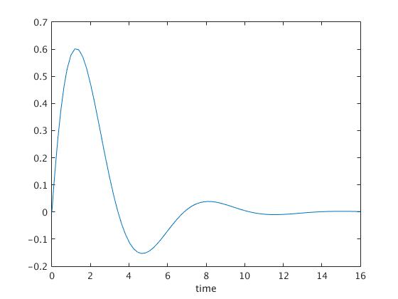
    function circuitequation
    
    %initial conditions are taken -1, and 0 (for simplicity)
    [t_1,y_1] = ode45(@circuit,[0 16], [-1 0]);
    
    plot(t_1,y_1(:,2),'b');hold on
    hold off
    
    xlabel('time');
    ylabel('Current, I');
    
    function dy = circuit(t,y)
    dy = zeros(2,1);
    dy(1) = y(2);
    dy(2)=-(2*.4*y(2))-(1*1*y(1)); 
    %here a is set to .4 but can be set to any value as long as that value corresponds to the same value for a in the initial conditions section of simplecircuit.m
    end
    end


    General Solutions of Homogeneous ODE

    Let us see how we can solve a first order ODE subject to an initial condition. In general, it will be in the form:

    \[ \begin{cases} y' &= f(t,y) , \quad t\in (t_0 , T) , \\ y(t_0 ) &= y_0 , \end{cases} \]
    for some known quantities \( \texttt{f}, t_0 , \texttt{T}, y_0 . \)

    Example. Let us solve the initial value problem

    \[ \begin{cases} y' &= 6t-3y+5 , \quad t\in (0 , 1) , \\ y(0 ) &= 3 . \end{cases} \]
    Since the slope function \( f(t,y) = 6t-3y+5 \) is a linear function, its solution is known
    \[ y(t) = 2\,e^{-3t} +2t +1 . \]

    The following matlab code numerically solves the given initial value problem with \( \texttt{ode45} \) and plot it on the same axis along with the exact solution.

    
      close all
      % define anonymous function/slope f(t,y)
      f = @(t,y) 6*t -3*y +5;
      % call ode45
      [t,y] = ode45(f, [0,1],3);
      % plot numerical solution and exact solution 
      plot(t, y, 'b-', t, 2*exp(-3*t)+2*t+1, 'r:');
      legend('numerical', 'exact', 'Location', 'best');
      legend boxoff
      shg
    Example here
    Reduction of order

    Using \( \texttt{ode45} \) to solve a higher order ordinary differential equation (ODE) requires a little pre-processing because it can only solve first order equations or system of equations.


    Variation of parameters

    Example. Find the general solution to:

    \[ 4x^2 y''(x) -12x\,y' (x) +16\,y(x) = x^4 \ln (x) , \quad x>0. \]
    Solution:

    The solution will be of the form

    \[ y(x) = y_h (x) + y_p (x) , \]
    where \( y_p (x) \) is a particular solution to the given nonhomogeneous differential equation, and \( y_h (x) \) is the general solution of the homogeneous equation corresponding to the given driven equation. To find \( y_h (x) ,\) we need to solve the homogeneous equation
    \[ 4x^2 y''(x) -12x\,y' (x) +16\,y(x) = 0 , \quad x>0. \]
    Since this is an Euler equation, we make make the substitution \( y (x) = x^p . \) Subsitution into the homegeneous equation yields
    \begin{align*} & 4x^2 p(p-1) \,x^{p-2} -12xp\,x^{p-1} + 16\, x^p =0 , \\ & 4x^p p(p-1) - 12p\,x^p + 16\,x^p =0 , \\ &4p(p-1) -12p + 16 =0 , \\ &4 \left( p-2 \right)^2 =0 \\ & p=2 \qquad (\mbox{of multiplicity 2}). \end{align*}
    Therefore, the homogeneous equation has two linearly independent solutions: \( y_1 (x) = x^2 \) and \( y_2 (x) = x^2 \ln x, \quad x>0. \) So
    \[ y_h (x) = C_1 y_1 (x) + C_2 y_2 (x) = C_1 x^2 + C_2 x^2 \ln x , \]
    where \( C_1 , \ C_2 \) are arbitrary constants. Now we find a particular solution \( y_p (x) \quad x>0. \) to the given driven equation in the form
    \[ y_p (x) = A(x)\, y_1 (x) + B(x)\, y_2 (x) = A(x)\, x^2 + B(x)\, x^2 \ln x \]
    using variation of parameters. To find the expressions of functions \( A(x) , \ B(x), \) we set up a Lagrange system of algebraic equations with respect to derivatives of unknown yet functions:
    \begin{align*} A' (x)\, x^2 + B' (x) \,x^2 \ln x &=0 , \\ A' (x)\, 2x + B' (x) \left[ 2x\,\ln x + x \right] &= \frac{x^4}{4}\, \ln x . \end{align*}
    From this system, we immediately find \( B'(x) = \frac{x}{4}\, \ln x, \) which we use to determine another varibale \( A'(x) = -\frac{x}{4}\, \ln^2 x. \) Integrating using the following matlab code,
    syms A(x) B(x) x 
    A(x) = int(1/4*x*(log(x)^2)
    B(x) = int(-1/4*x*log(x))
    we find a particular solution
    \[ y_p (x) = A(x)\, y_1 (x) + B(x)\, y_2 (x) = \frac{1}{16} \, x^4 \ln x \left( 1 - 2\,\ln x \right) -\frac{x^4}{16} \left( 2\,\ln^2 x -2\,\ln x +1 \right) . \]
    Final simplified solution:
    \[ y_p (x) = \frac{x^4}{16} \left( \ln x -1 \right) + C_1 x^2 + C_2 x^2 \ln x. \]
    syms x r y(x) y_h(x) y_p(x) y_1(x) y_2(x) c_1 c_2 p(x) f(x)
    p(x) = 4*x^2 % variable coefficient on second-order term
    f(x) = x^4*log(x) % right-hand side of equation to solve
    eqn = p(x)*diff(y_h(x),2) - 12*x*diff(y_h(x)) + 16*y_h(x) == f(x) % full equation to solve
    y(x) = y_h(x) + y_p(x)
    y_h(x) = x^r % substituion to solve Euler equation
    eqn_h = p(x)*diff(y_h(x),2) - 12*x*diff(y_h(x)) + 16*y_h(x) == 0 % Euler equation
    eqn_r = simplify(eqn_h) % yields condition for r
    r = solve(eqn_r,r) % yield vector of 2 values for r
    if r(1) ~= r(2) % if 2 distinct roots
        y_1(x) = x^r(1)
        y_2(x) = x^r(2)
    elseif r(1) == r(2) % if double root
        y_1(x) = x^r(1)
        y_2(x) = log(x)*x^r(1)
    end
    y_h(x) = c_1*y_1(x) + c_2*y_2(x) % general solution to homogeneous equation
    LaGrange = [y_1(x) y_2(x) 0; diff(y_1(x)) diff(y_2(x)) f(x)/p(x)] % Lagrange condition in matrix form
    LaGrange_sol = rref(LaGrange) % finds A_prime and B_prime by reducing Lagrange matrix
    A_prime(x) = LaGrange_sol(1,3)
    B_prime(x) = LaGrange_sol(2,3)
    A(x) = int(A_prime,x)
    B(x) = int(B_prime,x)
    y_p(x) = A(x)*y_1(x) + B(x)*y_2(x)
    y(x) = y_p(x) + y_h(x)


    Method of undetermined coefficients
    Operator method
    Numerical solutions

    Using \( \texttt{ode45} \) or \( \texttt{ode23} \) to solve a second order ordinary differential equation (ODE) requires a little pre-processing because it can only solve first order equations. Therefore, we need to modify our second order problem into equivalent first order problem. Consider the general second order differential equation in normal form subject to the initial conditions:

    \[ \begin{cases} y'' + p(t)\,y' + q(t)\,y &= f(t,y) , \quad t\in (t_0 , T) , \\ y(t_0 ) &= y_0 , \\ y' (t_0 ) &= v_0 . \end{cases} \]
    Typically, we set the new variables:
    \[ \begin{cases} y_1 &= y , \\ y_2 &= y' , \end{cases} \]
    which leads to the following system of differential equations involving \( y_1 \) and \( y_2 \) (but not \( y \) ):
    \[ \begin{cases} y'_1 & = y_2 , y'_2 &= f(t,y) - p(t)\,y_2 - q(t)\,y_1 , \quad t\in (t_0 , T) , \\ y_1 (t_0 ) &= y_0 , \\ y_2 (t_0 ) &= v_0 . \end{cases} \]
    This problem can be solved with \( \texttt{ode45} \) because it contains a system of first order differential equations. To rewrite it in a vector form, we introduce two vectors \( {\bf Y} = \begin{bmatrix} y_1 \\ y_2 \end{bmatrix} \) and \( {\bf F}(t, {\bf Y} ) = \begin{bmatrix} y_2 \\ f(t,y) - p(t)\,y_2 - q(t)\,y_1 \end{bmatrix}, \) which leads to
    \[ \begin{cases} {\bf Y}' &= {\bf F} (t, {\bf Y}) , \quad t\in (t_0 , T) , \\ {\bf Y} (t_0 ) &= \begin{bmatrix} y_0 \\ v_0 \end{bmatrix} . \end{cases} \]
    Now we get the expressions needed as inputs \( \texttt{ODEFUN} = {\bf F} \) and \( \texttt{Y0} = {\bf Y} (t_0 ) \) to invoke \( \texttt{ode45}. \) Since they are 2-column vectors, this will require some caution.

    Example 1.4.2: Let us solve the initial value problem involving the Airy functions:

    \[ \begin{cases} y'' &= x\,y , \quad x\in (0 , 1) , \\ y(0 ) &= y_0 , \\ y' (0) &= v_0 . \end{cases} \]
    Its solution is expressed through two Airy functions, commonly denoted as Ai(x) and Bi(x):
    \[ y (x) = \frac{y_0}{2}\,\Gamma \left( \frac{2}{3} \right) \left[ 3^{2/3} \mbox{Ai}(x) + 3^{1/6} \mbox{Bi} (x) \right] + \frac{v_0}{2}\, \Gamma \left( \frac{1}{3} \right) \left[ 3^{-1/6} \mbox{Bi}(x) - 3^{1/3} \mbox{Ai}(x) \right] . \]
    If we take \( y_0 = \mbox{Ai}(0) = 3^{-2/3}/\Gamma \left( \frac{2}{3} \right) \) and \( v_0 = \mbox{Ai}(0) = -3^{-1/3}/\Gamma \left( \frac{1}{3} \right) ,\) its solution becomes \( y(x) = \mbox{Ai}(x) . \)


    The equivalent first order system of differential equations will be
    \[ \begin{cases} {\bf Y}' = \begin{bmatrix} y_2 \\ x\,y_1 \end{bmatrix} = {\bf F} (t, {\bf Y}) , \quad t\in (t_0 , T) , \\ {\bf Y} (0 ) = \begin{bmatrix} y_0 \\ v_0 \end{bmatrix} . \end{cases} \] The following block of matlab code solves this vector equation subject to the initial conditions numerically with \( \texttt{ode45} \) and plot it on the same eaxis with the exact solution.
    
      close all
      % define anonymous function/slope F(x,Y)
      F = @(x,Y) [Y(2); t.*Y(1)];
      % call ode45
      [x,Y] = ode45(F, [0,1],[airy(0);airy(1,0)]);
      % plot numerical solution and exact solution 
      plot(x, Y(;,1), 'b-', x, airy(x), 'r:');
      legend('numerical', 'exact', 'Location', 'best');
      legend boxoff
      shg


    Applications ssss
    Pendilum equation

    There seems no doubt that the first person who investigated and established the mathematical theory and properties of the pendulum was Christiaan Huygens (this spelling of his name is taken from the title of his 1658 book Horologium Oscillatorium), the Dutch philosopher.

    For a point pendulum supported by massless, inextensible cord of length \( \ell ,\) the equation of motion for oscillations in a vacuum is

    \begin{equation} \label{E15.1} \ddot{\theta} + \left( g/\ell \right) \sin \theta =0 , \end{equation}
    where \( \ddot{\theta} = {\text d}^2 \theta / {\text d}t^2 , \) \( \omega_0^2 = g/\ell ,\) and g is gravitational acceleration. For infinitesimal displacements, we replace \( \sin\theta \) by \( \theta \) and the motion is simple harmonic with period
    \begin{equation} \label{E15.2} T_0 = 2\pi \left( \ell /g \right)^{1/2} = 2\pi / \omega_0 . \end{equation}
    A real pendulum bob has a finite size and the suspension wire has a mass. In addition, the wire connections to the bob and the support may have some structure. All such effects are encompassed in the physical pendulum equation for the period:
    \begin{equation} \label{E15.3} T = 2\pi \left( I/Mgh \right)^{1/2} , \end{equation}
    where I is the total moment of inertia about the axis of rotation, M is the total mass, and h is the distance between the axis and the center of mass. For the uniform spherical bob of radius a,
    \[ I= m\ell^2 \left[ 1 + \left( 2/5 \right) \left( a/\ell \right)^2 \right], \qquad M=m, \quad \mbox{and} \quad h =\ell . \]
    Qualitative analysis
    Applications