Return to computing page for the first course APMA0330
Return to computing page for the second course APMA0340
Return to computing page for the fourth course APMA0360
Return to Mathematica tutorial for the first course APMA0330
Return to Mathematica tutorial for the second course APMA0340
Return to Mathematica tutorial for the fourth course APMA0360
Return to the main page for the course APMA0330
Return to the main page for the course APMA0340
Return to the main page for the course APMA0360
Introduction to Linear Algebra with Mathematica
where subscripts indicate partial derivatives. For example, \( \displaystyle \quad u_t = \frac{\partial u}{\partial t} . \quad \)
The heat equation contains (phisical) real parameters, so α > 0 and γ ≥ 0.
All functions in the heat equation \eqref{eqHeat.1}, boundary condition \eqref{eqHeat.2}, and the initial condition \eqref{eqHeat.3} are assumed to be in the Hilbert space ℌ². Also all derivatives (ut, uxx) are assumed to be continuous in the open domain 0 < x < ∞, 0 < t < ∞
Example 1:
Let us consider the heat equation on
the half-line (0, ∞) with homogeneous boundary conditions:
If the solution to the above mixed initial/boundary value problem exists, then we know that it must be
unique from an application of the maximum principle. In terms of the heat conduction, one can think of
u in (1.1) as the temperature in an infinite rod, one end of which is kept at a constant zero temperature.
The initial temperature of the rod is then given by u₀(x).
Our goal is to solve the IBVP (1.1), and derive a solution formula, much like what we did for the heat
IVP on the whole line. But instead of constructing the solution from scratch, it makes sense to try to
reduce this problem to the IVP on the whole line, for which we already have a solution formula. This is
achieved by extending the initial data u₀(x) to the whole line. We have a choice of how exactly to extend
the data to the negative half-line, and one should try to do this in such a fashion that the boundary
condition of (1.1) is automatically satisfied by the solution to the IVP on the whole line that arises from
the extended data. This is the case, if one chooses the odd extension of φ(x), which we describe next.
By definition, a function ψ(x) is odd, if ψ(−x) = −ψ(x). But then plugging in x = 0 into this definition, one gets ψ(0) = 0 for any odd function. Recall also that the solution u(x, t) to the heat IVP with
odd initial data is itself odd in the x variable. This follows from the fact that the sum [u(x, t) + u(−x, t)]
solves the heat equation and has zero initial data, hence, it is the identically zero function by the uniqueness of solutions. Then, by our above observation for odd functions, we would have that u(0, t) = 0 for
any t > 0, which is exactly the boundary condition of (1.1)
This shows that if one extends u₀(x) to an odd function on the whole line, then the solution with the
extended initial data automatically satisfies the boundary condition of (1.1). Let us then define
\[
\mathfrak{\phi_{\mathrm{odd}}}(x) = \begin{cases}
u_0 (x), &\quad\mbox{for }\ x> 0 ,
\\
- u_0 (-x), &\quad\mbox{for }\ x< 0 ,
\\
0, &\quad\mbox{for }\ x = 0.
\end{cases}
\]
It is clear that φodd is an odd function, since we defined it for negative x by reflecting the u₀(x) with respect
to the vertical axis, and then with respect to the horizontal axis. This procedure produces a function
whose graph is symmetric with respect to the origin, and thus it is odd. One can also verify this directly
from the definition of odd functions. Now, let v(x, t) be the solution of the following IVP on the whole line
\[
\begin{cases}
v_t &= \alpha\,v_{xx} , \qquad -\infty < x < \infty , \quad 0 < t < \infty ,
\\
v(x,0) &= \mathfrak{\phi_{\mathrm{odd}}}(x) , \qquad -\infty < x < \infty .
\end{cases}
\tag{1.2}
\]
From previous section we know that the solution to (1.2) is given by the formul
\[
v(x,t) = \int_{-\infty}^{+\infty} S(x-\xi , t)\,\mathfrak{\phi_{\mathrm{odd}}}(\xi )\,{\text d}\xi , \quad t > 0,
\]
where the kernel is
\[
S(x,t) = \frac{1}{\sqrt{4\pi\alpha t}}\, e^{- x^2/(4\alpha t)}
\]
Restricting the x variable to only the positive half-line produces the function
\[
u(x,t) = v(x,t) \big\vert_{x\ge 0} .
\]
We claim that this u(x, t) is the unique solution of IBVP (1.1). Indeed, u(x, t) solves the heat equation
on the positive half-line, since so does v(x, t). Furthermore,
\begin{align*}
v(x,t) &= \int_0^{\infty} S(x-\xi , t) \,\mathfrak{\phi_{\mathrm{odd}}}(\xi )\,{\text d}\xi + \int_{-\infty}^0 S(x-\xi , t) \,\mathfrak{\phi_{\mathrm{odd}}}(\xi )\,{\text d}\xi
\\
&= \int_0^{\infty} S(x-\xi , t) \,u_0 (\xi )\,{\text d}\xi - \int_{-\infty}^0 S(x-\xi , t) \,u_0 (-\xi )\,{\text d}\xi .
\end{align*}
Making the change of variables ξ ↦ −ξ in the second integral on the right hand-side, and flipping the integration
limits gives
\[
v(x,t) = \int_0^{\infty} S(x-\xi , t) \,u_0 (\xi )\,{\text d}\xi - \int_{-\infty}^0 S(x+\xi , t) \,u_0 (\xi )\,{\text d}\xi
\]
Using definition of ϕodd and the above expression for v(x, t), as well as the expression of the heat kernel S(x, t), we can write the solution formula for the IBVP (1) as
\[
u(x,t) = \frac{1}{\sqrt{4\pi\alpha t}} \int_0^{\infty} \left[ e^{(x-\xi )^2 /(4\alpha t)} - e^{(x+\xi )^2 /(4\alpha t)} \right] u_0 (\xi )\,{\text d}\xi .
\tag{1.3}
\]
The method used to arrive at this solution formula is called the method of odd extensions or the reflection
method. We can make a physical sense of formula (1.3) by interpreting the integrand as the contribution
from the point ξ minus the heat loss from this point due to the constant zero temperature at the endpoint.
■
End of Example 1
To solve the given initial boundary value problem, we use sine Fourier transformation. So we multiply the differential equation \eqref{eqHeat.1} and the initial condition \eqref{eqHeat.3} by sine (kx) and integrate with respect to x from 0 to ∞. This results in the equation
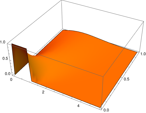
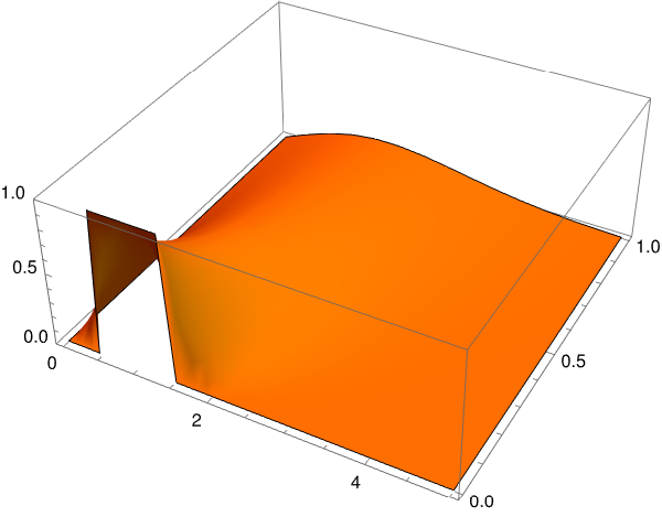
As it is seen from the graph, the corresponding integral I0(x, t) is unbounded at x = 0. To check the problem, we consider another initial function that vanishes at the origin:
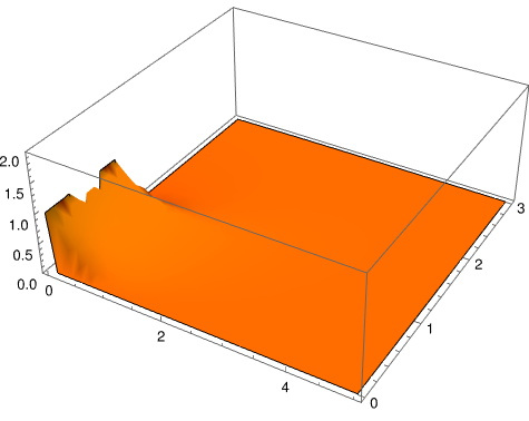
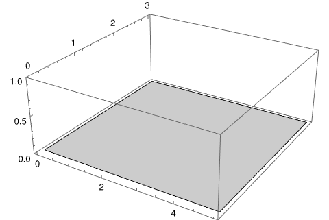
For numerical integration, we intrduce ε = 0.1 amd integrate with respect to τ from 0 to t − ε because the integrand approach 0 exponentially near τ = t; so
Boyd, J.P. and Flyer, N., Compatibility conditions for time-dependent partial differential equations and the rate of convergence of Chebyshev and Fourier spectral methods, Computer Methods in Applied Mechanics and Engineering, 1999, Volume 175, Issues 3–4, Pages 281--309. https://doi.org/10.1016/S0045-7825(98)00358-2
Chatziafratis, A., Boundary behaviour of the solution of the heat equation on the half line via the Fokas unified transform method, 2024,
https://doi.org/10.48550/arXiv.2401.08331
Chatziafratis, A., Fokas, A., Aifantis, E.C., Variations of heat equation on the half-line via the Fokas method, 2024,
First published: 08 September 2024
https://doi.org/10.1002/mma.10303
Chatziafratis, A., Mantzavinos, D., Boundary behavior for the heat equation on the half-line, 2022, https://doi.org/10.1002/mma.8245
Return to Mathematica page
Return to the main page (APMA0340)
Return to the Part 1 Basic Concepts
Return to the Part 2 Fourier Series
Return to the Part 3 Integral Transformations
Return to the Part 4 Parabolic PDEs
Return to the Part 5 Hyperbolic PDEs
Return to the Part 6 Elliptic PDEs
Return to the Part 6P Potential Theory
Return to the Part 7 Numerical Methods