Return to computing page for the first course APMA0330
Return to computing page for the second course APMA0340
Return to computing page for the fourth course APMA0360
Return to Mathematica tutorial for the first course APMA0330
Return to Mathematica tutorial for the second course APMA0340
Return to Mathematica tutorial for the fourth course APMA0360
Return to the main page for the course APMA0330
Return to the main page for the course APMA0340
Return to the main page for the course APMA0360
Introduction to Linear Algebra with Mathematica
Glossary
Preface
1D Third kind IBVPs for heat equation
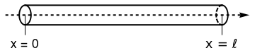
Figure below depicts a thin, uniform rod of length ℓ oriented along the x-axis so that the left end of the rod corresponds with the origin. At time t = 0, the rod has a known temperature distribution as a function of x ∈ [0, ℓ] that is denoted by f(x), 0 ≤ x ≤ ℓ. This distribution represents the initial condition (IC) for the for the model. Additionally, the temperature boundary conditions (BC) at x = 0 and x = ℓ are specified for all time t ≥ 0.
right1 = Graphics[{Thick, Circle[{1, 0}, {0.03, 0.05}, {-Pi/2, Pi/2}]}];
right2 = Graphics[{Thick, Dashed, Circle[{1, 0}, {0.03, 0.05}, {Pi/2, 3*Pi/2}]}];
line1 = Graphics[{Thick, Line[{{0, 0.05}, {1, 0.05}}]}];
line2 = Graphics[{Thick, Line[{{0, -0.05}, {1, -0.05}}]}];
arrow = Graphics[{Thick, Dashed, Arrow[{{-0.1, 0}, {1.14, 0}}]}];
lineL = Graphics[{Line[{{0, 0}, {0, -0.1}}]}];
lineR = Graphics[{Line[{{1, 0}, {1, -0.1}}]}];
tl = Graphics[{Black, Text[Style["x = \[ScriptL]", 18, FontFamily -> "Mathematica1"], {1.0, -0.15}]}];
t0 = Graphics[{Black, Text[Style["x = 0", 18], {0.0, -0.15}]}];
Show[left, right1, right2, line1, line2, arrow, lineL, lineR, tl, t0]
Under the assumption that the rod is "narrow" so that the spacial dependence of temperature is in terms of x only, the governing PDE for temperature is one-dimensional heat equation ut = α uxx. (A careful derivation of this equation is provided in the first section.) The objective is to determine the function u(x, t) that satisfy the PDE, initial and boundary conditions. This is an example of an initial boundary value problem (IBVP).
We consider the IBVP with the boundary conditions of the third kind:
All these conditions guarantee that the formulated IBVP is well-posed, which means that its solution is unique, exists, and continuously depends on parameters. Problems that are not well-posed in the sense of Hadamard are termed ill-posed. For example, the inverse heat equation, deducing a previous distribution of temperature from final data, is not well-posed in that the solution is highly sensitive to changes in the final data. Also, if regulariry conditions are violated, the problem becomes an ill-posed and some kind of regularization will be needed.