Return to computing page for the first course APMA0330
Return to computing page for the second course APMA0340
Return to computing page for the fourth course APMA0360
Return to Mathematica tutorial for the first course APMA0330
Return to Mathematica tutorial for the second course APMA0340
Return to Mathematica tutorial for the fourth course APMA0360
Return to the main page for the course APMA0330
Return to the main page for the course APMA0340
Return to the main page for the course APMA0360
Introduction to Linear Algebra with Mathematica
Fourier series analysis requires utilization of Hilbert spaces that are a more natural environment for approximation and expansion of functions with respect to eigensystems. As such, we present the main ingredients that are needed to understand this topic.
Our motivation to study Hilbert spaces in this section stems from a necessity to extend Euclidean space to an infinite dimensional case. Roughly speaking, a Hilbert space is an infinite dimensional (complete) version of Euclidean space.
Vector Space
It is assumed that you are already familiar with vector spaces, so we will just provide a friendly refresher on this topic. The definition of vector spaces involves the set of reals or complex numbers, which are both fields and serve as the set of scalars. We recall their notations:
ℝ = all real numbers;
ℂ = all complex numbers, so ℂ = {𝑎 + jb | 𝑎, b ∈ ℝ}, where j is the imaginary unit, i.e., j² = −1.
A vector space (also called a linear space) consists of a set V (elements of V are traditionally
called vectors), a field of scalars (real or complex), and two operations
An internal operation called vector addition that for two vectors v, w ∈ V assigns a third vector, written v + w ∈ V
An outer operation called scalar multiplication that takes a scalar c ∈ F (either ℝ or ℂ) and
a vector v ∈ V, and produces a new vector, written c v ∈ V.
These two operations satisfy the following conditions (called axioms).
Associativity of vector addition: (u + v) + w = u
+ (v + w) for all u, v, w ∈ V.
Commutativity of vector addition: u + v = v
+ u for all u, v ∈ V.
Existence of a zero vector: There is a vector in V, written 0 and called
the zero vector, which has the property that u + 0 = u for all u ∈ V.
Existence of negatives: For every u ∈ V, there is a vector in
V, written −u
and called the negative of u, which has the property that u + (−u) = 0.
Associativity of multiplication: (𝑎b)u = 𝑎(bu) for any scalars 𝑎, b and any vector u.
Distributivity: (𝑎 + b)u = 𝑎u +
bu and 𝑎(u + v) = 𝑎u + 𝑎v for all scalars 𝑎, b and all vectors u, v ∈ V.
𝑎, b ∈ F (= ℝ or ℂ) and
Unitary: 1u = u for every vector u ∈ V.
Most likely you are familiar with finite dimensional vector spaces (that contain finite number of linearly independent vectors) such as ℝn or ℂn. However, we are heading towards infinite dimensional spaces.
Convex Sets
Let V be a vector space. A subset C ⊂ V is
called convex if
\[
t\,x + \left( 1-t \right) y \in C \qquad\mbox{for} \quad
\forall x,y \in C \quad \mbox{and} \quad 0 \leqslant t \leqslant 1.
\]
This means that the segment that connects any two points in C is in C. Differently stated, for all t ∈ [0,1]:
\[
t\,C + \left( 1-t \right) C \subseteq C .
\]
Lemma 1:
For any collection of sets {Cα} and {Dα} and every t ∈ ℝ:
Theorem 1 (Convexity is closed under intersections):
Let V be a vector space that contains a collection (not necessarily
countable) of convex subsets
{Cα} ⊂ V for all α ∈ A. Then
\[
C = \cap_{\alpha \in A} C_{\alpha}
\]
is convex.
For all t ∈ [0,1]:
\begin{align*}
t \, C + \left( 1- t \right) C &= t \cap_{\alpha \in A} C_{\alpha} + \left( 1- t \right) \cap_{\alpha \in A} C_{\alpha}
\\
&= \cap_{\alpha \in A} t\,C_{\alpha} + \cap_{\alpha \in A} \left( 1- t \right) C_{\alpha}
\\
& \subseteq \cap_{\alpha \in A} \left( t\, C_{\alpha} + \left( 1- t \right) C_{\alpha} \right)
\\
& \subseteq \cap_{\alpha \in A} C_{\alpha} =C .
\end{align*}
Another proof. Let x, y ∈ C. By definition,
\[
x, y \in C_{\alpha} \qquad\mbox{for all} \quad \alpha \in A.
\]
Since all the Cα are convex,
\[
\left( t\,x + (1-t)\, y \right) \in C_{\alpha} \qquad\mbox{for all} \quad \alpha \in A \quad\mbox{and} \quad t \in [0,1] .
\]
Interchanging the order of the quantifiers, we obtain
\[
\left( t\,x + (1-t)\, y \right) \in C \qquad\mbox{for all} \quad t \in [0,1] .
\]
Theorem 2 (Convex sets are closed under convex linear combinations):
Let V be a vector space that contains a convex subset
C ⊂ V. Then for every
(x1, … , xn) ⊂ C and every non-negative (t1, … , tn) real numbers that sum up to 1
\[
\sum_{i=1}^n t_i x_i \in C.
\]
Equation
\[
\sum_{i=1}^n t_i x_i \in C.
\tag{1.1}
\]
holds for n = 2 by the definition of convexity. Suppose
(1.1) were true for n = k. That is, for elements x₁, x₂, … , xk from C and for nonnegative scalars t₁, t₂, … , tk that sum to 1, \( \displaystyle \sum_{i=1}^k t_i = 1 , \) we have
define \( \displaystyle t = \sum_{i=1}^k t_i . \)
Let us consider two cases, when t = 0 and when t ≠ 0. If t = 0, then tk+1 = 1 and \( \displaystyle \sum\limits _{i=1}^{k+1}t_i x_i = t_{k+1}x_{k+1}=x_{k+1}\in C . \) When t ≠ 0, we can write
\[
\sum_{i=1}^{k+1} t_i x_i = \sum_{i=1}^{k} t_i x_i + t_{k+1} x_{k+1} = t \sum_{i=1}^{k} \frac{t_i}{t}\, x_i + \left( 1- t \right) x_{k+1} \in C.
\]
Normed and Metric Spaces
A normed vector space or normed space is a vector space V over the real or complex numbers that is equipped with a function called a norm on V ∥ ∥ : V → ℝ+ that satisfies the following four conditions:
It is nonnegative, meaning that ∥x∥ ≥ 0 for every vector x ∈ V.
It is positive on nonzero vectors, that is,
\[
\| x \| = 0 \qquad\Longrightarrow \qquad x=0.
\]
For every vector x, and every scalar α,
\[
\| \alpha\,x \| = |\alpha |\,\| x\| .
\]
The triangle inequality holds; that is, for every vectors x and
y,
\[
\| x+y \| \le \| x \| + \| y \| .
\]
We also need a more general set than a normed space.
A set X whose elements are called points is called a metric space
if to any two points x, y ∈ X there is associated a real number
d(x, y), called the
distance between x and y, such that for x, y, z ∈ X,
In 1906, Maurice Fréchet (1878--1973) introduced metric spaces in his work "Sur quelques points du calcul fonctionnel." However, the name "metric space" is due to Felix Hausdorff (1868--1942).
Every normed space is also a metric space because its norm
induces a distance, called its (norm) induced metric, by the formula
\[
d(x,y) = \| x-y \| .
\]
Example 1:
Let ℝn be an Euclidean space over the scalars ℝ, in which we introduce three norms:
Example 3:
Let [𝑎, b] be a finite interval of nonzero length, and consider
a set of functions defined on this interval. We introduce three norms in this vector space:
A set of functions for which norm (3.1) is finite is denoted by
𝔏¹([𝑎, b]) or simply 𝔏¹ or just 𝔏. Notation
L1 is also widely used; however, we prefer to utilize Gothic font for L because the latter usually denotes a linear operator in PDEs.
where square root denotes positive branch, so \( s^{1/2} = \sqrt{s} > 0 \quad \) for s > 0. The space of square integrable functions is denoted by 𝔏²([𝑎, b]) or simply 𝔏². Of course, integration in Eq.(3.2) should be considered in Lebesgue sense rather than Riemann one, but technical requirements of Lebesgue measurability will not be a concern for us.
Here ess sup means essential supremum; it is the sup of f over all but a set of measure zero.
Again, the measure theory won’t matter to us.
The space of bounded functions is denoted by 𝔏∞([𝑎, b]) or simply 𝔏∞. Notation
L∞ is also widely used; however, we prefer to use Gothic font for L because the latter usually denotes a linear operator.
The infinite norm is naturally applicable to the set of all continuous functions, usually denoted as ℭ[𝑎, b] or C[𝑎, b]. Then in this vector space,
Note that this nesting doesn’t hold when at least one of the bounds (𝑎 or b) is infinite.
■
Riemann Integral
Since Fourier coefficients for any function f are determined upon integration over the interval of definition, we are forced to take a closer look at integration. Historically, the first rigorous definition of the integral was made by Bernhard Riemann in his
paper "Über die Darstellbarkeit einer Function durch eine trigonometrische Reihe" (On the representability of a function by a trigonometric series),
published in 1868 in Abhandlungen der Königlichen Gesellschaft der Wissenschaften zu Göttingen.
The conventional Riemann integral is a much less flexible tool than the
integral of Lebesgue. The practical advantages have mostly to do with the
interchange of the integral with other limiting operations, such as sums,
other integrals, differentiation, and the like.
With the integral at hand, one can define an area of a plain object or a volume of a three-dimensional object. In this case, mathematicians say that you can define a measure---the most fundamental concept in Euclidean geometry.
In the classical approach to geometry, the measure of a body was often
computed by partitioning that body into finitely many components, moving around each component
by a rigid motion (e.g., a translation or rotation), and then reassembling
those components to form a simpler body which presumably
has the same area or volumse. However, you can come into trouble with a truncation approach, as the Banach-Tarski paradox shows that the
unit ball B := {(x, y, z) ∈ ℝ³ : x² + y² + z² ≤ 1} in three dimensions
can be disassembled into a finite number of pieces (in fact, just five
pieces suffice), which can then be reassembled (after translating and
rotating each of the pieces) to form two disjoint copies of the ball B.
To avoid such a situation, one should prohibit highly pathological partitions, which is always required.
Let [𝑎, b] be an interval of
positive length, and f : [𝑎, b] → ℝ be a function. A
tagged partition
P = {(x0, x1, . … , xn), (y1, y2, . … , yn)} of [𝑎, b] is a finite sequence of real
numbers 𝑎 = x0 < x1 < < xn = b, together with additional
numbers xi-1 ≤ yi ≤ xi for each i = 1, 2, … , n. We abbreviate xi − xi-1 as δxi. The quantity Δ(P) = sup1≤i≤n δxi will be called the norm of the tagged partition. The Riemann sum R(f, P) of f with respect to the tagged partition P is defined as
We say that f is Riemann integrable on [𝑎, b] if there exists a real number, denoted
\( \int_a^b f(x)\,{\text d}x \)
and referred to as the Riemann integral
of f on [𝑎, b], for which we have
for every tagged partition P with \( \Delta (P) \le \delta . \)
If [𝑎, b] is an interval of zero length, we adopt the convention that
every function f : [𝑎, b] → ℝ is Riemann integrable, with a Riemann
integral of zero.
■
Theorem 3:
A function f is Riemann integrable over [𝑎, b]
if and only if it is continuous almost
everywhere on [𝑎, b].
Proof of this theorem can be found in Chapter 5 (Theorem8) of Royden and Fitzpatrick book.
Hence, a real-valued function f
defined on some finite closed interval [𝑎, b] is Riemann integrable (which we abbreviate as integrable) if it is bounded, and if for every ε > 0, there is a subdivision [𝑎 = x0 < x1 < ··· < xN-1 < xN = b of the interval [𝑎, b], so that if
\[
U = \sum_{j=1}^N \left[ \sup_{x_{j-1} \le x \le x_j} f(x) \right] \left( x_j - x_{j-1} \right) , \qquad
L = \sum_{j=1}^N \left[ \inf_{x_{j-1} \le x \le x_j} f(x) \right] \left( x_j - x_{j-1} \right) ,
\]
then we have U−L < ε.
Such functions are bounded, but may have infinitely many discontinuities of measure zero.
A full course would be needed to develop Lebesgue integration theory properly. In this
subsection, we present only a brief sketch of the Lebesgue theory, with the focus on the
features most relevant for applications to PDEs.
The
reader who is content to take these statements as articles of faith may do
so; nice proofs and additional information can be found in Munroe [1953]
and Roydcn [I963]; for the more advanced student, Rudin [1966] and
Hewitt and Stromberg [1965] are suggested. The latter are modern presentations;
one of the oldest but most elementary and satisfactory explanations is given
by de la Vallée-Poussin [1950] (the first edition appeared in I916).
Henri Lebesgue.
Henri Léon Lebesgue (1875--1941)
was a French mathematician known for his theory of integration, which was a generalization of the 17th-century concept of integration—summing the area between an axis and the curve of a function defined for that axis. His theory was published originally in his dissertation Intégrale, longueur, aire ("Integral, length, area") at the University of Nancy during 1902.
Lebesgue entered the École Normale Supérieure in Paris in 1894 and was awarded
his teaching diploma in mathematics in 1897. He studied Baire’s papers on dis-
continuous functions and realized that much more could be achieved in this area.
Building on the work of others, including that of Émile Borel and Camille Jordan,
Lebesgue formulated measure theory, which he published in 1901. He generalized
the definition of the Riemann integral by extending the concept of the area (or
measure), and his definition allowed the integrability of a much wider class of
functions, including many discontinuous functions. This generalization of the
Riemann integral revolutionized integral calculus. Up to the end of the nineteenth
century, mathematical analysis was limited to continuous functions, based largely
on the Riemann method of integration.
After he received his doctorate in 1902, Lebesgue held appointments in regional
colleges. In 1910 he was appointed to the Sorbonne, where he was promoted to
Professor of the Application of Geometry to Analysis in 1918. In 1921 he was
named as Professor of Mathematics at the Collège de France, a position he held
until his death in 1941. He also taught at the École Supérieure de Physique et de
Chimie Industrielles de la Ville de Paris between 1927 and 1937 and at the École
Normale Supérieure in Sèvres.
Since 1868, mathematicians introduced many other definitions of integration and corresponding measures. However, Riemann integration dominates in all applications and we will use his definition in most cases. However, there exists another version of integration that plays an important role in probability theory, real analysis, and many other fields in mathematics. In 1904 while lecturing at the Collège de France, Henri Lebesgue (1875–1941) introduced the integral that now bares his name.
Now is right time to answer your curious question: why do you need to learn more sophisticated definition of an integral although it is hard to find its practical applications in numerical analysis? There are a couple of reasons to study Lebesgue integration. First, I want to confuse you---otherwise you will think that the course is too light. Second, you should be prepared for other courses that may require Lebesgue integration. Third, PDEs involve special function spaces that utilize Lebesgue integration. Moreover, in this course, we will use a space of square integrable functions, and this set becomes a Hilbert space only when integration is performed via Lebesgue, not Riemann.
Convergence questions for Fourier series have been historically an important motivation for developing entire branches of analysis, such as Lebesgue integration theory and functional analysis.
Thus, Henri Lebesgue developed a new generalization of Riemann integration in which the focus was on the range of the function, instead of
on the domain. The distinction between the two approaches can be
seen by envisioning the graph of a real function f whose range is the
reals. Whereas Riemann focuses on partitioning the x-axis, Lebesgue’s
integral partitions the ordinate instead. That is, Riemann partitions the
domain of f into a finite number of intervals and on each interval approximates the values that f takes. Using the rectangles generated by
the product of the value of the function on each interval and the length
of that interval, Riemann approximates the area under the function.
Lebesgue, on the other hand, partitions the range of the function into
a finite number of intervals, and for each partition chooses a value to
”represent” the function for that partition on his approximation (call
it s) (so for all x in the partition, s(x) equals the representative). s is
called a simple function, which means it has a finite range.
Not every function is Lebesgue integrable and some restrictions will be necessary. To get a sense of the kinds of functions that are integrable,, we recall the characteristic function (or indicator function) of a set S ⊆ X is the function
\[
\chi_S (x) = \begin{cases} 1, & \quad\mbox{if} \quad x \in S , \\
0, & \quad \mbox{otherwise}.
\end{cases}
\]
If E ⊆ X is a measarable set, it seems intuitive that the integral of χE should be the same as the measure of E. However, if S ⊆ X is a non-measarable set, then the same intuition suggests that we should not be able to assign a value to the integral of χS. A linear finite combination of indicator functions is called a simple function, which is assumed to be Lebesgue integrable.
It is clear that Lebesgue integration needs to construct some sort of
manner of measuring the area of very complicated set. In particular, one needs to approximate sets of the form { x | f(x) ∈ [𝑎, b] } for some real numbers 𝑎, b. So Lebesgue defines a measure of such sets, denotes it by m. The first step is to consider simple functions, functions that have only finite discrete range of values.
Let g be a simple measurable function on a m-measurable
set E = ∐Ei and g(x) = 𝑎i for x ∈ Ei. Then define the
Lebesgue integral of g over E:
\[
\int_E g = \sum_i a_i m\left( E_i \right)
\]
A measurable function f ≥ 0 on a measurable set E is integrated as
\[
\int_E f = \sup_{0 \le s \le f} \int s .
\]
This definition shows that initially Lebesgue integral is defined for nonnegative functions. Since every real-valued function can be represented by a difference of such functions,
provided that at least one of ∫ f+ and ∫ f- is less than infinity. If both are less
than ∞, f is said to be “summable." Notice that f is summable iff |f| is so. The integral of f times the indicator function χB of a measurable set B⊂E is declared to be the “integral of f over B."
The final step for definition of
the Lebesgue integral uses the following idea: the limit
of integrals of simple functions should be the integral of the limit of these functions. In other words, for any function f that is approximated by a sequence of simple functions { fn }, we have
This equality holds true in the Riemann sense too, but under less mild
conditions. Eq.\eqref{EqLebesgue.1} is crucial when an "arbitrary" function is approximated by simple functions. We say that a function f is Lebesgue integrable if and only if there exists a sequence of simple functions {gₙ} such that
\( \sum_{n\ge 1} \int g_n < \infty . \)
\( f(x) = \sum_{n\ge 1} g_n (x) \quad \) almost everywhere (so it holds for all the sets which have non-zero measures).
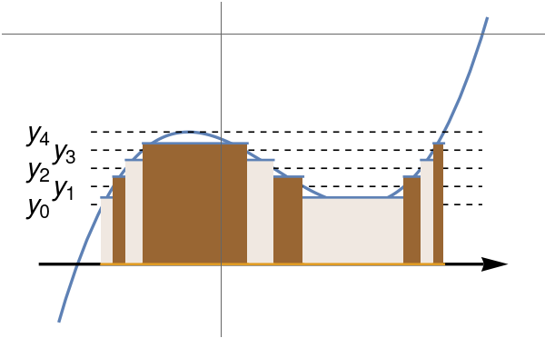
Approximation of the Lebesgue integral \( \displaystyle \int_{-3}^5 \left( x-5 \right) \left( x^2 + 2x+5 \right) {\text d}x \) using simple functions is given below. Lebesgue’s recipe tells you first to subdivide the vertical axis by a series
of points
\[
\sum_{k=1}^n \xi_{k-1} \,\times \,\mbox{measure of } \left\{ x \,:\, y_{k-1} \leqslant f(x) \leqslant y_k \right\} ,
\]
in which ξk-1 is any point from the closed interval [yk-1, yk] and measure { x : ··· } is the sum of the lengths of the subintervals of 𝑎 ≤ x ≤ b on which the stated inequality takes place. Finally, we claim that
this sum approaches some number denoted by
\[
\int_a^b f(x)\,{\text d} x
\]
as n ↑ ∞ and the biggest of the lengths yk − yk-1 (k ≤ n) tends to zero,
We extend the idea of measure from unions of disjoint subintervals to the wider class of “measurable” subsets of the interval 𝑎 ≤ x ≤ b in order
to integrate a much wider class of functions by means of Lebesgue's
recipe than you can by Riemann's.
Theorem 4:
If a function f is Riemann integrable over finite interval [𝑎, b],
then it is Lebesgue integrable, and both integrals are equal.
The next item has a more formal explanation of the Lebesgue integral. Fix
an interval Q ⊂ ℝ¹, which may be bounded (—oo < 𝑎 ≤ x ≤ b < ∞), or a
half-line (—oo < 𝑎 ≤ x < ∞), or the whole line (−∞ <x < ∞), and let us
agree that the measure of a (countable) union of nonoverlapping intervals is
the sum of their lengths, finite or not; in particular, we ascribe to a single point
or any countable family of points measure 0. This definition of measure
may now be extended to the class of “Borel measurable” sets. This is the
smallest collection of subsets of Q that contains all subintervals of Q and
is closed under countable unions, countable intersections, and complementation. It turns out that if you require the extended measure of a countable
union of disjoint “Borel measurable” sets to be the sum of their individual
measures, then you can do this in only one way. A small additional extension
(to the class of “Lebesgue measurable” sets) is made for technical convenience by throwing in any subset of a “Borel-measurable” set of measure
0 and ascribing to it measure 0 also. This second extension is the Lebesgue
measure; from now on “measurable” always means “Lebesgue measurable.”
The straight forward way of expressing the Lebesgue measure is by the following recipe: for any measurable set E,
in which the infimum is taken over the class of countable coverings of E by
means of internals In so \( \displaystyle E \subset \cup_{n\ge 1} I_n . \) You can also use supremum instead of infinimum when intervals are inscribed into E,
Theorem 5:
Every countable set has measure 0 (almost everywhere zero).
We attempt to integrate the Dirichlet function on [0, 1]. Actually, it is a indicator function of the set of irrational numbers.
Why is the Dirichlet function not Riemann integrable? Using the Riemann approach, we partition the domain into equal length subintervals, since the Dirichlet function is not continuous in each subinterval, then the supremum in each subinterval is always one, as well as the infimum of the upper Riemann sum, and the infimum in each subinterval is always zero, as well as the supremum of the lower Riemann sum. Therefore, the lower Riemann sum is zero while its upper Riemann sum is 1. It’s not Riemann intergrable.
Then why is it Lebesgue integrable? To answer this, we apply Theorem 5.
The key observation tells us that
the set of real or irrational numbers has a larger cardinality than the set of all the rational numbers or natural numbers, this is proved by Cantor. Therefore, an interval of real numbers is very dense. If we take out all the rational numbers away from this interval, the size of the interval doesn’t change. Like taking away the resolved substance from the water doesn't really change the volume.
Apparently, the Lebesgue measure of the whole interval [0, 1] is the same as the Lebesgue measure of the set of irrational numbers inside this interval and equals to 1. As a result, the Lebesgue integral of the Dirichlet function on [0, 1] is 1.
End of Example 4
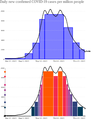
Let us determine the cumulative COVID-19 case count from a graph of smoothed new daily cases (left). Two graphs represent Riemann (top) vs Lebesgue (bottom) integration for determination of cumulative function (Summer-Fall 2021, Serbia).
Incidentally, an improper Riemann integral is not always the same thing as a Lebesgue integral.
In particular,
Lebesgue integration may not be suitable for improper integration involving Cauchy principal value regularization.
Example 5:
For example, sinc(x) is not Lebesgue integrable, but it is integrable according to Riemann:
\[
\int_{-\infty}^{+\infty} \frac{\sin x}{x} {\text d} x =
2\int_0^{\infty} \frac{\sin^{+} x}{x} {\text d} x - 2\int_0^{\infty} \frac{\sin^{-} x}{x} {\text d} x = \infty - \infty
\]
However, \( \displaystyle \int_{-\infty}^{+\infty} \frac{\sin x}{x} \, {\text d} x = \pi , \) as Mathematica confirms:
Integrate[Sin[x]/x, {x, -Infinity, Infinity}]
End of Example 5
A real-valued function f on some interval Q is measurable if { x : α ≤ f(x) ≤ β } is a measurable set for every choice of α and β in Q. The integral of a nonnegative measurable
function f is now defined by forming the Lebesgue-type sums
and making n↑∞ with the understanding that 0×∞ = 0. As n increases,
the subdivision k/2n (k≥ 0) becomes finer and finer, and the sums increase
to a finite or infinite limit, which is declared to be the Lebesgue integral of f:
\[
\int_{Q} f = \int_a^b f = \int_a^b f(x)\,{\text d} x .
\]
To sum up, the Lebesgue integral of a nonnegative function always exists,
although it may be +∞.
Generalizing the dot product in
the Euclidean space ℝn that was originally introduced by the ancient Greek mathematician Euclid in his treatise Elements (Ancient Greek: Στοιχεῖα Stoikheîa), we
consider the inner product in ℂn defined by
where asterisk or overline is used for complex conjugate:
\[
z^{\ast} = \overline{z} = \left( a + {\bf j} b \right)^{\ast} = a - {\bf j} b , \qquad {\bf j}^2 = -1.
\]
As usual, j denotes the imaginary unit at ℂ, so j² = −1. There is no universal notation for inner product; in mathematics, it is denoted with comma: ⟨ x , y ⟩, while in physics, the inner product involves vertical bar: ⟨ x | y ⟩. This reflects Dirac's notation to denote by ⟨ v | a vector, called a ket. Then the inner product of the vectors ⟨ v | with |w〉 is written ⟨ v | w ⟩. In this case, vector ⟨ v | is considered as the bra vector, that is, the functional.
Therefore, both inner product notations will be utilized in future to please everyone.
An inner product space is a vector space V over the field F of scalars (ℝ or ℂ) together with an inner product, that is a function
\[
\langle \cdot , \cdot \rangle \, : \,V\times V \mapsto F (= \mathbb{R} \quad\mbox{or}\quad \mathbb{C})
\]
that satisfies the following three properties for all vectors x , y , z
∈ V and all scalars 𝑎, b ∈ F.
Conjugate symmetry:
\[
\langle x , y \rangle = \langle y , x \rangle^{\ast} = \overline{\langle y , x \rangle} = \langle x \,|\, y \rangle .
\]
\[
\langle a\,x + b\,y\,,\, z\rangle = a \langle x\,,\, z\rangle + b \langle y\,,\, z\rangle .
\]
Positive-definiteness: if x is not zero, then
\[
\langle x \,,\,x \rangle = \langle x \,\vert\,x \rangle > 0 \qquad \mbox{for} \quad x \ne 0.
\]
Physics consists of more than mathematics: along with mathematical symbols one always has a
“physical picture,” some sort of intuitive idea or geometrical construction that aids in thinking about what
is going on in more approximate and informal terms than is possible using “bare” mathematics. There are two types of vectors in Dirac notation: the bra vector | v ⟩ and the ket vector ⟨ w |, serving as a functional. In quantum mechanics, their inner product ⟨ w | v ⟩ implies that the probability of measuring the state | v ⟩ to be | w ⟩ is |⟨ w | v ⟩|².
Conjugate symmetry implies that ⟨ x , x ⟩ is always a real number. If F is ℝ, conjugate symmetry is just symmetry.
The inner product induces a natural norm via
\begin{equation} \label{EqNorm.7}
\| x \| = \langle x\,,\, x\rangle^{1/2} = \langle x\,|\, x\rangle^{1/2} = \| x \|_2 .
\end{equation}
As usual, the square root in the equation above is a positive branch of the analytic function defined by \( s^{1/2} = \sqrt{s} > 0 \) for positive s. With this norm, every inner space becomes a normed space and a metric space with the distance:
\[
d(x,y) = \| x - y \| = \langle x-y\,, \, x-y \rangle^{1/2} .
\]
Lemma (Cauchy--Bunyakovsky--Schwarz (CBS) inequality):
For any two vectors u and v from a space with inner product, the following CBS-inequality holds:
\[
\vert \left\langle u \,,\, v \right\rangle \vert \leqslant \left\langle u \,,\, u \right\rangle^{1/2} \cdot \left\langle v \,,\, v \right\rangle^{1/2} = \| u \| \cdot \| v \| ,
\]
with equality holding in the CBS inequality if and only if u and v are linearly dependent.
The CBS inequality for sums was published by the French mathematician and physicist Augustin-Louis Cauchy (1789--1857) in 1821, while the corresponding
inequality for integrals was first proved by the Russian mathematician Viktor Yakovlevich Bunyakovsky (1804--1889) in 1859. The modern proof
(which is actually a repetition of the Bunyakovsky's one) of the integral inequality was given by the German mathematician Hermann Amandus Schwarz (1843--1921) in 1888.
Assuming that v ≠ 0, we have the identity:
\[
\frac{1}{\| v \|^2} \,\left\| \| v \|^2 u - \langle u, v \rangle\,v \right\|^2 = \| u \|^2 \| v \|^2 - \left\vert \langle u, v \rangle \right\vert^2
\tag{CBS.1}
\]
Because the left hand side of Eq. (CBS.1) is non-negative, so is the right hand side, which proves the CBS inequality.
Lemma (parallelogram identity):
For any two vectors u and v from a space with inner product, the following parallelogram identity holds:
\[
\| u + v \|^2 + \| u - v \|^2 = 2 \left( \| u \|^2 + \| v \|^2 \right) .
\]
For every u, v ∈ X, we have
\[
\| u \pm v \|^2 = \| u \|^2 + \| v \|^2 \pm \Re \langle u, y \rangle .
\]
The parallelogram identity follows by adding both equations.
Two vectors x and y are called orthogonal iff their inner product is zero:
\[
\langle x\,,\,y \rangle = \langle y\,,\,x \rangle = 0 \qquad \iff \qquad x \perp y .
\]
A set of vectors { xi } is called orthogonal iff every element of this set is orthogonal to all other elements.
A sequence x1, x2, x3,
… in a metric space (X, d) is called Cauchy if for every positive real number r > 0 there is a positive integer N such that for all positive integers m, n > N,
\[
d(x_m , x_n ) < r .
\]
Every convergent sequence is Cauchy, but the converse is not always true.
Theorem 6:
The limit of a convergent sequence in a metric space is unique.
Suppose that { xn } is a sequence in a metric space (X, d) that converges to x and y. Choose ϵ > 0. There are N and M such that d(xn, x) < ϵ for n ≥ N and d(xm, y) < ϵ for m ≥ M. Hence, for
d(xn, y) ≤ ϵfor n ≥ M. Hence, for n ≥ max(N, M), we have
A metric space (X, d) is complete if every Cauchy sequence of points in X has a limit that is also in X.
The name "complete" was introduced in 1910 by the famous Russian mathematician Vladimir Steklov (1864--1926).
Theorem 7:
Let X be an inner-product vector space. Then,
there exists a Hilbert space ℌ such that
There exists a linear injection T ∶ X → ℌ that preserves the inner-product \( \displaystyle \quad \langle x\,,\,y \rangle_X = \langle T\,x\,,\,T\,y \rangle_{ℌ} \quad \) for all x, y ∈ X (i.e., elements in X can be identified
with elements in ℌ).
Image(T) is dense in ℌ (i.e., X is identified with “almost all of" ℌ).
Moreover, the inclusion of X in ℌ is unique: For any linear inner-product preserving injection T1 ∶ X → ℌ1, where ℌ1 is a Hilbert space and Image(T1) is dense in ℌ1, there is a linear isomorphism S ∶ ℌ → ℌ1, such that T1 = S ○ T (i.e.,
ℌ and ℌ1 are isomorphic in the category of inner-product spaces).
We start by defining the space ℌ. Consider the set of Cauchy sequences
{xn} in X. Two Cauchy sequences {xn} and {yn} are said to be equivalent (denoted {xn} ∼ {yn}) if
\[
\lim_{n\to\infty} \| x_n - y_n \| = 0.
\]
It is easy to see that this establishes an equivalence relation among all Cauchy sequences in X. We denote the equivalence class of a Cauchy sequence {xn} by [xn], and define ℌ as the set of equivalence classes.
We endow ℌ with a vector space structure by defining
It remains to show that ⟨ ⋅,⋅ ⟩ℌ is indeed an inner product (do it).
The next step is to define the inclusion T : X → ℌ. For x ∈ X, we set
\[
T\, x = \left[ (x, x, x, \ldots ) \right] .
\]
In other words, T maps every vector in X into the equivalence class of a constant sequence. By the definition of the linear structure on Hilbert space ℌ, T is a linear transformation. So it is preserves the inner-product as
\[
\langle T\, x\,\vert\, T\, y \rangle = \lim_{n\to\infty} \left\langle (T\,x)_n , (T\,y)_n \right\rangle_X = \lim_{n\to\infty} \left\langle x , y \right\rangle_X = \left\langle x , y \right\rangle_X .
\]
The next step is to show that Image(T) is dense in ℌ. Let h ∈ ℌ and let {xn} be a
representative of h. Since {xn} is a Cauchy sequence in X,
which proves that Txn → h, and therefore
Image(T) is dense in ℌ.
The next step is to show that ℌ is complete. Let {hn} be a Cauchy sequence in ℌ. For every n, let {xn,k} be a Cauchy sequence in X in the equivalence class of hn.
Since Image(T) is dense in ℌ, there exists for every n an element yn ∈ X, such that
The last step is to show the uniqueness of the completion modulo isomorphisms. Let h ∈ ℌ. Since Image(T) is dense in ℌ, there exists a sequence {yn} ⊂ X such that
It follows that {T yn} is a Cauchy sequence in ℌ, and because T preserves the
inner-product, {yn} is a Cauchy sequence in X. It follows that {T1 yn} is a Cauchy
sequence in ℌ1, and because the latter is complete, {T1 yn} has a limit in ℌ1. This
limit is independent of the choice of the sequence {yn}, hence it is a function of h,
which we denote by
\[
S(h) = \lim_{n\to\infty} T_1\,y_{n} .
\]
We leave it as an exercise to show that S satisfies the required properties.
For every metric space X, there exists a complete metric space Y
such that X is dense in Y.
Let Ω be a bounded set in ℝn and let \( \displaystyle W = \overline{\Omega} \) be its closure (Ω together with its boundary). For example, if Ω = [1, 2) is a semiclosed interval, then its closure is [1, 2]. We denote by ℭ(W) the set of continuous complex-valued functions on its closure. This space is made into a complex vector
space by pointwise addition and scalar multiplication
where asterisk or overline indicates a complex conjugate.
The corresponding norm in ℭ(W) is induced by the inner product:
\[
\| f \| = \left( \int_{\Omega} \vert f(x) \vert^2 {\text d} x \right)^{1/2} .
\]
This space is not complete.
Example 6:
We present some examples that lead you to believe that completeness is possible in a way that the original normed space is dense in in more wider complete space.
The set of real numbers ℝ is the completion of the rational numbers ℚ, where the metric on both spaces is induced by the absolute value function.
The vector space of continuous functions ℭ[𝑎, b] is the completion of the set of polynomials, where the metric on both spaces is induced by ∥ ∥∞ = sup | |.
The space 𝔏¹[𝑎, b] of Lebesgue integrable functions on finite interval [𝑎, b] is the completion of the space of continuous functions ℭ[𝑎, b], where norm is
\[
\| f(x) \| = \int_a^b | f(x) |\,{\text d} x \qquad \mbox{or more generally} \qquad \int_a^b | f(x) |\,w(x)\, {\text d} x
\]
for some positive integrable function w, called weight.
End of Example 6
To clarify the importance of completeness, let us consider an example of convergence of a sequence of rational numbers { bn } that is generated by conditionally convergent series
where εn becomes as small
as we wish (although usually not zero) with growing n. So ln(2) is an abbreviation of the limit of the sequence---its precise numerical value is unknown (it is an irrational number) but can be approximated with any accuracy you want. We do not discuss an issue that this limit, ln(2), depends on how numerical values of the elements bn are evaluated. It is well-known that by rearranging terms within every partial sum bn we can obtain any number as the limit---this is the reason why numerical evaluation of this series is an ill-posed problem.
Hence, proving the convergence of the sequence of rational numbers { bn } becomes problematic because we don't know exactly the numerical value of ln(2). Its numerical value remains transcendental quantity in the sense that we can never obtain it with full accuracy
(we can operate with it, however, as a symbolic unchangeable
quantity, independent of the never ending limit process). But in
this case we must give a criterion for the existence of a limit that
makes no use of the (practically not available) quantity ln(2)∈ℝ. We must completely rely on the sequence b₁, b₂, b₃, … . It was the French mathematician Augustin-Louis Cauchy who
in his book Cours d'Analyse (1821) suggested a proof of sequence convergence based on the property
that holds for all n > N and all finite m ≥ 1. Therefore, considering sequences in a complete metric space, we can prove their convergence based on Cauchy convergence test without any knowledge what the limit is.
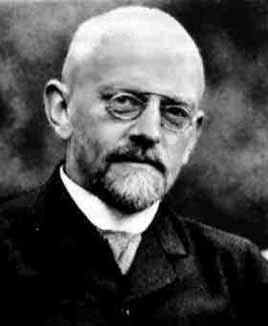
Hilbert spaces are named after David Hilbert (1862--1943)---a German mathematician who was said to know all mathematics. The name "Hilbert space" was introduced in 1929 by the «father of
computers» John von Neumann,
who most clearly recognized the importance of Hilbert spaces as a result of his seminal work on the foundations of quantum mechanics, where the state of a physical system is represented by a vector in a Hilbert space.
David Hilbert’s parents were Otto Hilbert, who was a judge, and Maria Therese Erdtmann. His father came from a legal family, while his mother’s family were merchants. Both families were Protestant, and his father was devoted to his faith. It was Maria Therese’s interests that shaped the young boy’s curiosity---she was an enthusiastic amateur mathematician and astronomer.
Hilbert’s famous twenty-three Paris problems challenged (and still today
challenge) mathematicians to solve fundamental questions. Hilbert’s famous
speech The Problems of Mathematics was delivered to the Second International
Congress of Mathematicians in Paris. It was a speech full of optimism for
mathematics in the coming century, and he felt that open problems were the sign
of vitality in the subject. Hilbert’s problems included the continuum hypothesis,
Goldbach’s conjecture, and the Riemann hypothesis.
David's remarks characterize him precisely:
Mathematics knows no races or geographical boundaries; for mathematics, the cultural world is one country.
and
No one shall expel us from the paradise that Cantor has created for us.
In 1930 Hilbert retired but only a few years later, in 1933, life in Göttingen changed completely when the Nazis came to power and Jewish lecturers were dismissed. By the autumn of 1933 most had left or were dismissed. Hilbert, although retired, had still been giving a few lectures. In the winter semester of 1933-34 he gave one lecture a week on the foundations of geometry. After he finished giving this course he never set foot in the Institute again. In early 1942 he fell and broke his arm while walking in Göttingen. This made him totally inactive and this seems to have been a major factor in his death a year after the accident.
A Hilbert space ℌ is a real or complex inner product space that is also a complete metric space with respect to the distance function induced by the inner product; \( \displaystyle d(x,y) = \| x - y \| = \langle x-y, x-y \rangle^{1/2} . \)
Its counterpart for normed space deserves a special attention.
A normed vector space that is complete is called the Banach space.
Banach spaces are named after the Polish mathematician Stefan Banach (1892--1945), who introduced this concept and studied it systematically in 1920s.
Example 7:
Let us consider the space of Lebesgue integrable functions on compact interval [𝑎, b]. This space is denoted by 𝔏¹[𝑎, b] or simply 𝔏 (note that notation L¹ is also widely used). The norm in 𝔏¹[𝑎, b] is introduced by the integral
\[
\| f(x) \| = \int_a^b | f(x) |\,{\text d} x \qquad \mbox{or more generally} \qquad \int_a^b | f(x) |\,w(x)\, {\text d} x
\]
for some positive integrable function w, called weight. The Banach space of integrable functions with weight w is denoted by 𝔏¹([𝑎, b], w). Mathematicians show that the space is complete when integration is understood in the Lebesgue sense, so it is an example of a Banach space.
Example 8:
We know from calculus that if a sequence { fn(x) } of continuous functions from finite closed interval [𝑎, b] to ℝ converges uniformly to f(x), then f is continuous on this interval. We are going to formalize this statement by introducing the space of continuous functions, denoted as ℭ[𝑎, b], and introducing the uniform norm:
\[
\| f(x) \| = \sup_{x\in [a,b]} | f(x)| .
\]
Recall: the supremum of a set is the least upper bound of the set, a number
M such that no element of the set exceeds M, but for any
positive ε, there is a member of the set which exceeds M −ε,
However, if interval [𝑎, b] is bounded, which we assume, the supremum can be replaced by the maximum according to the Weierstrass extreme value theorem.
It is not hard to verify that ℭ[𝑎, b] is a vector space.
It is fairly straightforward to show that the supremum norm satisfies the following properties:
∥f∥∞ ≥ 0 for all continuous functions;
∥f∥∞ = 0 if and only if f(x) ≡ 0;
∥λ · f∥∞ = |λ| · ∥f∥∞;
∥f + g∥∞ ≤ ∥f∥∞ + ∥g∥∞.
Suppose that a sequence { fn(x) } of continuous functions converges uniformly to f. Then for any positive ε we can find an
N such that for all x in the interval,
We need to show that for such sequence there exists an f such that
\[
\forall \varepsilon > 0, \quad \exists N \in \mathbb{N} \quad \mbox{such that} \quad \| f_n (x) - f(x) \|_{\infty} < \varepsilon \quad \forall n \ge N.
\]
For each fixed x in the interval [𝑎, b], we have that
|fn(x) −fm(x)| < ε for m, n greater than some N.
Thus, each ( fn(x) }n∈ℕ is a Cauchy sequence in ℝ. Now since ℝ is complete, there is a limit of this sequence in ℝ. We’ll call this
\( \displaystyle f(x) = \lim_{n\to\infty} f_n (x) . \)
Now we need to show that this sequence converges uniformly.
Since fn is a Cauchy sequence, there is a value of N,
independent of x, such that
\[
| f_n (x) - f_m (x)| < \varepsilon , \qquad \forall n,m \ge N \qquad \Longrightarrow \qquad | f(x) - f_m (x)| < \varepsilon , \quad \forall m \ge N \quad \forall x \in [a,b] .
\]
Therefore, sequence { fm } converges to f uniformly.
Since f is the uniform limit of continuous functions, f itself is continuous.
So now we have seen that ℭ[𝑎, b] is a complete, normed vector space. We
can now think of two functions f and g as vectors in an abstract vector space,
with a notion of distance between the two functions given by the sup-norm of
the difference f − g.
End of Example 8
In the theory of quantum mechanics, the configuration space of a system has the structure of a vector
space, which means that linear combinations of states are again allowed states for the system (a fact
that is known as the superposition principle). More precisely, the state space is a so-called Hilbert space.
A Hilbert space is called separable if it contains a countable dense subset.
In a space with inner product (also referred to as pre-Hilbert space or Euclidean space) one can introduce orthogonality between two vectors. This definition is crucial for Riesz representation theorem.
Two vectors x and y from a vector space with inner product X
are called orthogonal if ⟨x | y⟩ = 0. We will abbreviate it as x ⊥ y.
Let M be a subset of some vector space X with inner product. We denote by M⊥ a set of all vectors from X that are orthogonal to every element from M.
A sequence {ϕn} of orthogonal vectors in Hilbert space ℌ is called an orthogonal basis or complete
orthogonal system for ℌ if the only vector f that is orthogonal to to all elements of the sequence, ⟨ f , ϕn⟩ = 0, is zero, f = 0.
Note that the word “complete” used here does not mean the
same thing as completeness of a metric space.
Theorem 8:
An orthogonal sequence {ϕn} of vectors of a separable Hilbert space is complete
if and only if there is no nonzero vector orthogonal to all the functions ϕn.
Let f be an element of a Hilbert space ℌ, and let {ϕn} be a sequence of orthogonal elements in ℌ.
Let \( \displaystyle s_n = \sum_{k=1}^n c_k \phi_k \) be the n-th least-square approximation to f by a linear combination of ϕ₁, ϕ₂, … , ϕn. We know that \( \displaystyle s_n = \sum_{k=1}^n c_k \phi_k \) be the n-th least-square approximation, \( \displaystyle c_k = \langle f, \phi_k \rangle / \langle \phi_k , \phi_k \rangle , \) and for m > n,
According to Bessel's inequality, the series above of positive numbers is convergent; hence, the last sum in the preceding display tends to zero as n → ∞.
That is, the sequence {sn} is a Cauchy sequence.
It follows that ℌ, being complete, contains a vector s to which the sn
converge; let h = f − s = \( \displaystyle \lim_{m\to \infty} \left( f - s_m \right) . \) Then, since
\( \displaystyle \langle f- s_m , \phi_k \rangle = 0 \) for all m ≥ k, we have in the limit, as m → ∞, ⟨ h, ϕk ⟩ = 0 for all k.
According to Riesz--Fischer theorem,
a sequence {ϕn} of orthogonal elements of a Hilbert vector space ℌ
is complete if and only if the Parseval equality holds for all f in ℌ:
This assures that h = 0 for all f if and only if {ϕn} is complete.
Riesz representation theorem:
Let λ be a bounded linear
functional on a Hilbert space ℌ. Then there exists a unique element y ∈ ℌ such
that λ(x) = ⟨x, y⟩ for all x ∈ ℌ. Furthermore, ‖λ‖ = ‖y‖.
This spectacular statement was published by Frigyes Riesz (Sur une espèce de géométrie analytique des systèmes de fonctions sommables, Comptes rendus de l'Académie des Sciences, 1907, 144, pp. 1409–1411) in the very same issue of the
Comptes Rendus by Maurice Fréchet (Sur les ensembles de fonctions et les opérations linéaires, Les Comptes rendus de l'Académie des sciences, 1907, 144, pp. 1414–1416) and is now called (or should be called) the
Fréchet--Riesz theorem.
If λ = 0, take y = 0. Otherwise, let M = Ker(λ); M is a closed subspace of
ℌ because M = λ−1(0), and M ≠ ℌ because λ ≠ 0. By the projection theorem in section v,
ℌ = M ⊕ M⊥. Pick a nonzero element z ∈ M⊥. Then λ(z) ≠ 0, and, by replacing
z with z/λ(z), we may assume that λ(z) = 1. For x ∈ ℌ, x = x − λ(x)z + λ(x)z. It
is easy to verify that w = x − λ(x)z ∈ M.
Observe that ⟨x, z⟩ = ⟨w, z⟩ + ⟨λ(x)z, z⟩ = λ(x)‖z‖². Define y = z/‖z‖². Then,
by the above identity,
\( \displaystyle \lambda (x) = \frac{\langle x, z \rangle}{\| z \|^2} = \langle x, y \rangle . \)
To prove that y is unique, suppose
that there is another element y1 ∈ ℌ such that ⟨x, y⟩ = ⟨x, y1⟩ for all x ∈ ℌ. Then
⟨x, y − y1⟩ = 0 for all x ∈ ℌ. Choose x = y − y1. Then ‖y − y1‖² = 0; hence y = y1.
Finally, |λ(x)| = |⟨x, y⟩| ≤ ‖x‖‖y‖. Thus ‖λ‖ ≤ ‖y‖.
Also |λ(y)| = |⟨y, y⟩| = ‖y‖² = ‖y‖‖y‖. This shows that ‖λ‖ ≥ ‖y‖ and that
‖λ‖ = ‖y‖ .
Examples of Hilbert spaces
There are really three ‘types’ of separable Hilbert spaces (over either ℝ or ℂ). The finite dimensional
ones, essentially just ℝn or ℂn, with which you are pretty familiar and two infinite dimensional cases corresponding to being separable (having a countable dense subset) that are isomorphic (they are in 1-1 correspondence). As we shall see, there is really only one separable infinite-dimensional Hilbert
space and that is what we are mostly interested in. Nevertheless some proofs (usually the nicest ones) work in the non-separable case too.
If there is a 1-1 map of a set A onto a set B, then we say that
A and B are in 1-1 correspondence, have the same cardinality or cardinal
number, or are equivalent, and we write A ∼ B.
Our first vector space to be considered is the space of
sequences, or of signals in discrete-time
The vector operations on these
sequences are performed term-by-term, so that a + b is the sequence [a₀ + b₀, a₁ + b₁, a₂ + b₂, a₃ + b₃, …]
We consider only such sequences for which the following norm is finite
where square root is defined by a positive root branch. The set of such sequences is denoted by ℓ2 or ℓ². More precisely, this space is denoted by ℓ²(ℕ) because its indices are nonnegative integers. It turns out that the ℓ2 norm is generated by the inner product:
\[
\left\langle x \,\vert\, y \right\rangle = \sum_{i\ge 0} x_i^{\ast} y_i = \sum_{i\ge 0} \overline{x_i} \, y_i = \left\langle x \,,\, y \right\rangle .
\]
In mathematics, it is common to define the inner product by applying the complex conjugate to the second argument:
\[
\left\langle x \,,\, y \right\rangle = \sum_{i\ge 0} x_i \, y_i^{\ast} = \sum_{i\ge 0} x_i \, \overline{y_i} = \left\langle x \,\vert\, y \right\rangle .
\]
This definition is equivalent to the previous definition, which is used in physics and engineering.
Theorem 9:
Any infinite-dimensional separable Hilbert space ℌ is isomorphic to ℓ², that is, there exists a linear map
\[
T\,:\,ℌ \mapsto \ell^2
\]
which is 1-1, onto, and satisfies \( \displaystyle \langle T\, u \,|\,T\,v \rangle_{\ell^2} = \langle u \,|\,v \rangle_{ℌ} \quad \) and \( \displaystyle \quad \| T\,u \|_{\ell^2} = \| u \|_{ℌ} \quad \) for all u, v ∈ ℌ.
Choose an orthonormal basis { ϕn }, which exists and set
This maps ℌ into ℓ² by Bessel’s inequality. Moreover, it is linear since the entries
in the sequence are linear in u. It is 1-1 since Tu = 0 implies
⟨u | ϕn⟩ = 0 for all n; this leads to u = 0 by the assumed completeness of the orthonormal basis. It is surjective because if \( \displaystyle \quad \left\{ c_n \right\} \in \ell^2 , \quad \) then
\[
u = \sum_n c_n \phi_n
\]
converges in ℌ. This is the same argument as above – the sequence of partial sums
is Cauchy since if n > m,
Again, by continuity of the inner product, T u = { ci }, so T is surjective.
The equality of the norms follows from equality of the inner products and the
latter follows by computation for finite linear combinations of the ϕn and then in
general by continuity.
Actually, there is another version of ℓ²(ℤ) space that is equivalent to the one defined previously. It is also denoted by ℓ² or ℓ2 and consists of all sequences of the form
It turns out that the ℓ2 or ℓ2 norm is generated by the inner product:
\[
\left\langle x \,\vert\, y \right\rangle = \sum_{i=-\infty}^{\infty} x_i^{\ast} y_i = \sum_{i=-\infty}^{\infty} \overline{x_i} \, y_i = \left\langle x \,,\, y \right\rangle .
\]
A relation ∼ that satisfies the following properties is called equivalence relation.
A ∼ A (reflexive);
A ∼ B ⇔ B ∼ A (symmetric);
If A ∼ B and B ∼ C, then A ∼ C (transitive).
Our next and the most important example of Hilbert spaces is 𝔏²([𝑎, b], w) or simply 𝔏²[𝑎, b] when either w(x) is known or w = 1. This is the class of functions with which Fourier series and/or integrals are
most naturally associated and therefore plays a central role in everything
to follow.
The space 𝔏²[𝑎, b] consists of all equivalent classes of (measurable) functions that are square integrable (in Lebesgue sense, but we will always consider Riemann integrals because we avoid pathological cases). Hence, elements or vectors in 𝔏²[𝑎, b] represent equivalence classes of functions; so f ∼ g iff f(x) = g(x)
almost everywhere (up to a set of measure zero; roughly speaking, when these functions differ at discrete number of points). We are forced to use equivalent classes of functions because integrals do not see the difference between functions that are almost everywhere equal. From this point of view, the Heaviside function H(t) and the unit functions u(t) are equivalent in 𝔏²(−∞, ∞):
In other words, two functions are equivalent iff (= if and only if)
\[
\int_a^b \left\vert f(x) - g(x) \right\vert^2 {\text d}x = 0 \qquad \mbox{or for the space with weight function:} \qquad \int_a^b \left\vert f(x) - g(x) \right\vert^2 w(x)\,{\text d}x = 0
\]
The inner product in 𝔏²([𝑎, b], w) is defined by
\[
\left\langle f \,\vert\, g \right\rangle = \int_a^b f(x)^{\ast} g(x)\,w(x)\,{\text d}x = \int_a^b \overline{f(x)}\, g(x)\,w(x)\,{\text d}x = \left\langle f \,,\, g \right\rangle ,
\]
where asterisk or overline stands for complex conjugate. Based on this definition of inner product with weight function w(x) > 0, we introduce the norm in
𝔏²([𝑎, b], w) by
\[
\| f \|_2 = \sqrt{\left\langle f \,\vert\, f \right\rangle} = \left( \int_a^b
\left\vert f(x) \right\vert^2 w(x)\,{\text d}x \right)^{1/2} ,
\]
where the radical stands for the positive branch of square root, so
\( \sqrt{z} > 0 \) for z > 0. Again, in mathematics, it is common to use the equivalent definition:
\[
\left\langle f \,,\, g \right\rangle = \int_a^b f(x) g(x)^{\ast}\,w(x)\,{\text d}x = \int_a^b f(x)\, \overline{g(x)}\,w(x)\,{\text d}x = \left\langle f \,\vert\, g \right\rangle ,
\]
The vector space ℭ[𝑎, b] of all continuous functions (either real or complex) on the closed interval [𝑎, b] is dense in
𝔏²[𝑎, b]. However, ℭ[𝑎, b] is not complete under the mean square norm; for instance, the sequence of continuous functions
\[
f_n (x) = \begin{cases}
1, & \quad | x - x_0 | \le r ,
\\
1 + n \left( r - | x - x_0 | \right) , & \quad r \le | x - x_0 | \le r + 1/n ,
\\
0, & \quad | x - x_0 | > 1 + 1/n ,
\end{cases}
\]
converges pointwise to the discontinuous function
\[
u(x) = \begin{cases}
1, & \quad | x - x_0 | \le r,
\\
0, & \quad | x - x_0 | > r.
\end{cases}
\]
The sequence { fn } is a Cauchy sequence because (for n > k)
which means that u = g almost everywhere, a contradiction.
The completion of ℭ[𝑎, b]
with respect to the square mean norm is isomorphic to the
Hilbert space 𝔏²[𝑎, b] of square integrable functions.
Theorem 10:
The space of square Lebesgue integrable functions 𝔏²[𝑎, b] on interval [𝑎, b] is a complete Hilbert space.
Proof of this statement can be found in Rudin's book, section 3.11. Mathematicians can prove Theorem 10 in one line: the dual space X* is complete for any normed space X. REmember that the dual space of 𝔏²[𝑎, b] is itself.
Example 9:
Let us consider a sequence of functions fn(x) = √n × χ[0, 1/n](x), where χA is the characteristic function of the set A so it is identically zero outside A. This sequence of functions converges pointwise to zero. However,
\[
\int_0^1 \left\vert f_n (x) \right\vert^2 {\text d} x = n \times (1/n) = 1 .
\]
Hence, the sequence { fn } does not converge in 𝔏²[0, 1].
Example 10:
Let ℛ denote the set of complex-valued Riemann integrable
functions on [0, 1].
This is a vector space over ℂ. Addition is defined pointwise by
\[
\left( f + g \right) (x) = f(x) + g(x) .
\]
Naturally, multiplication by a scalar λ ∈ ℂ is given by
An inner product is defined on this vector space by
\[
\left\langle f\,\vert\, g \right\rangle = \int_0^1 f(x)^{\ast} g(x)\,{\text d} x .
\]
The norm of f is then
\[
\| f \| = +\left( \left\langle f\,\vert\, f \right\rangle \right)^{1/2} = \left( \int_0^1 |f(x)|^2 {\text d} x \right)^{1/2} .
\]
One needs to check that the analogue of the Cauchy--Bunyakovsky--Schwarz and triangle inequalities hold in this example; that is,
|⟨ f , g ⟩| ≤ ∥f∥ ∥g∥ and ∥f + g∥ ≤ ∥f∥ + ∥g∥.
In order to show that the vector space of Riemann integrable functions ℛ is a Hilbert space, we have to show two conditions. The first is to show that the norm ∥⋅∥ is a positive-definite function.
The norm condition for a Hilbert space fails, since ∥g∥ = 0 implies only that g vanishes at its points of continuity. This is not a very serious limitation. One can get around the
difficulty that g is not identically zero by adopting the convention that
such functions are actually the zero function, since for the purpose of
integration, g behaves precisely like the zero function.
A more essential difficulty is that the space ℛ is not complete. One
way to see this is to start with the function
can easily be seen to form a Cauchy sequence in ℛ. However, this sequence cannot converge to an element in ℛ, since that limit,
if it existed, would have to be f. However, Mathematica knows how to evaluate this improper integral:
Integrate[Log[1/x], {x, 0, 1}]
1
Linear Operators in Hilbert space
In quantum mechanics, observables correspond to linear operators acting in a Hilbert space.
A linear operator A is a linear mapping of the Hilbert space ℌ:
\[
A : D(A) \subset ℌ \mapsto ℌ ,
\]
where D(A) is a linear subspace of ℌ, called the domain of A.
A linear operator A acting in a Hilbert space ℌ
is called bounded if
\[
\| A \| = \sup_{\| x \| = 1} \| A\,x \|
\]
is finite. If this is the case, ∥A∥ is called the (operator) norm of A.
Theorem 11:
A linear operator A is bounded if and only if A is continuous.
(⇒) For f, g ∈ D(A), let h = f − g with h₁ = h/∥h∥. Then
\[
\| A \left( f - g \right) \| = \left\| A \left( \| h \| \,h_1 \right) \right\| = \| h \| \,\| A\,h_1 \| \le \| h \| \,\| A \| .
\]
Thus, operator A is Lipschitz continuous.
(⇐) First note that since A is linear, we have A(0) = 0. From continuity at the zero vector, it follows that
there exists a positive δ such that ∥A(f)∥
= ∥A(f) − A(0)∥ ≤ 1 for every f from the Hilbert space having norm ∥f∥ ≤ δ. Hence, g ∈ ℌ with ∥g∥ = 1, then
The spectrum is a generalization of the notion of eigenvalues: If λ is an eigenvalue, then λ ∈ σ(A),
the converse, however, does not hold in general. This generalization is needed in quantum mechanics,
because unbounded operators might not have any eigenvalues at all, but the eigenvalues (or rather
spectral values) of an observable have a physical meaning, namely the possible results of a measurement
of that observable.
Theorem 12 (Uniform Boundedness Principle):
Let X be a Banach space and Y be a normed vector space, and let { Tα }α∈A be a family of bounded linear operators from X to Y. Then either
This principle is known also as the Banach–Steinhaus theorem. The theorem was first published in 1927 by Stefan Banach and Hugo Steinhaus, but it was also proven independently by Hans Hahn. A proof of this theorem can be found, for instance, in Rudin's book [Chapter 5].
Rather than study general distributions based on duality, we utilize their applications based on the Riesz representation theorem and corresponding convergence.
Let { xn } be a sequence of vectors in an inner-product space X. This sequence is said to be weakly convergent
to a vector x ∈ X if
\[
\lim_{n\to\infty} \langle x_n , y \rangle = \langle x , y \rangle \qquad\mbox{for any} \quad y \in X .
\]
Then the element x is called the weak limit of the sequence
{ xn }, which we denote as xn ⇀ x.
A sequence { xn } of vectors in an inner-product space X is said to be weakly Cauchy if the sequence of numbers
\[
\langle x_n , y \rangle
\]
is a Cauchy sequence for any y ∈ X.
If a sequence has a weak limit, then the weak
limit is unique, for if x and z are both weak limits of { xn }, then
\[
\lim_{n\to\infty} \langle x_n , y \rangle = \langle x , y \rangle = \langle z , y \rangle ,
\]
from which follows that x = z. Therefore, the weak limit is unique.
It is clear that any sequence that converges strongly (by norm) has the same weak limit because
\[
\lim_{n\to\infty} | f(x_n ) - f(x)| \le \lim_{n\to\infty} \| f \| \,\| x_n - x \| = 0
\]
Theorem 13:
A weak Cauchy sequence in a Hilbert space is bounded.
Recall that a sequence is weakly Cauchy if for every y ∈ ℌ, the inner products ⟨xn , y⟩
is a
Cauchy sequence, i.e., converges (but not necessarily to the same ⟨x , y⟩). For every
n ∈ ℕ, define the set
\[
V_n = \left\{ y \in ℌ : \forall k \in \mathbb{N}, \quad |\langle x_k , y \rangle | \le n \right\}
\]
These sets are increasing V₁ ⊆ V₂ ⊆ ··· . They are closed (by the continuity of the
inner product). Since for every y ∈ ℌ, the sequence { |⟨ xk , y ⟩| } is bounded,
\[
\forall y \in ℌ, \quad \exists n \in \mathbb{N} \qquad\mbox{such that } \quad y \in V_n ,
\]
i.e.,
\[
\cup_{n\ge 1} V_n = ℌ .
\]
There exists an m ∈ ℕ for which Vm contains a ball, say, B(y0, ρ) of radius ρ centered at
y0. That is,
\[
\forall y \in B(y_0 , \rho ) , \qquad \forall k \in \mathbb{N} , \qquad |\langle x_k , y \rangle | \leqslant m .
\]
\[
F(y) = \langle y , x \rangle = \lim_{n\to\infty} \langle y , x_n \rangle \qquad\mbox{for every} \quad y \in ℌ.
\]
We are going to prove that a unit ball in a Hilbert space is weakly sequentially compact. It is not true for strong convergence! Take for example
ℌ = ℓ² and xn = en (the n-th unit vector). This is a bounded sequence that does not
have any (strongly) converging subsequence. On the other hand, it has
a weak limit (zero).
Theorem 15:
Every
bounded sequence in a Hilbert space ℌ has a weakly converging subsequence. (Equivalently, the unit ball in a Hilbert space is weakly compact.)
We first prove the theorem for the case where ℌ is separable. Let {xn} be a
bounded sequence. Let {yn} be a dense sequence. Consider the sequence ⟨y1, xn⟩.
Since it is bounded, there exists a subsequence \( \displaystyle \left\{ x_n^{(1)} \right\} \)
of {xn} such that \( \displaystyle \left\langle y_1, x_n^{(1)} \right\rangle \)
converges. Similarly, there exists a sub-subsequence \( \displaystyle \left\{ x_n^{(2)} \right\} \) such that \( \displaystyle \left\langle y_2, x_n^{(2)} \right\rangle \)
converges (and also \( \displaystyle \left\langle y_1, x_n^{(2)} \right\rangle \) converges). We proceed inductively to construct the
subsequence \( \displaystyle \left\{ x_n^{(k)} \right\} \) for which all the \( \displaystyle \left\langle y_m, x_n^{(k)} \right\rangle \) for m ≤ k converge. Consider the
diagonal sequence \( \displaystyle \left\{ x_n^{(n)} \right\} , \) which is a subsequence of {xn}. For every k, \( \displaystyle \left\{ x_n^{(n)} \right\} \) has a
tail that is a subsequence of \( \displaystyle \left\{ x_n^{(k)} \right\} , \) from which follows that for every k,
Clearly, ℌ0 is a closed separable subspace of ℌ. Hence, there exists a subsequence {xn,k} of
{xn} that weakly converges in ℌ0, namely, there exists an x ∈ ℌ0 such that
\[
\lim_{n\to\infty} \langle y, x_n \rangle = \langle y, x \rangle
\]
for all y ∈ ℌ0 . Take y ∈ ℌ. From the projection theorem,
\[
y = \mathbb{P}_{ℌ_0} y + \mathbb{P}_{ℌ_{0}^{\perp}} y .
\]
So
\[
\lim_{n\to\infty} \langle y, x_n \rangle = \lim_{n\to\infty} \langle \mathbb{P}_{ℌ_{0}} y, x_n \rangle = \left\langle \mathbb{P}_{ℌ_{0}} y + \mathbb{P}_{ℌ_{0}^{\perp}} , x \right\rangle = \langle y , x \rangle .
\]
Weak convergence does not imply strong convergence, and does not even implies
a strongly convergent subsequence. The following theorem establishes another
relation between weak and strong convergence.
Theorem (Banach-Saks):
Let ℌ be a Hilbert space. If a sequence {xn} weakly converges to x, so xn ⇀ x,
then there exists a subsequence \( \displaystyle \left\{ x_{n_k} \right\} \) that is Cesàro summable:
Without loss of generality we may assume that x = 0, otherwise consider the sequence {xn −x}. As {xn} weakly converges, it is bounded; denote M = lim supn ∥ xn ∥.
We construct the subsequence \( \displaystyle \left\{ x_{n_k} \right\} \) as follows. Because xn ⇀ 0, we can choose \( \displaystyle \left\{ x_{n_k} \right\} \) such that
Show that this space is a real inner-product space.
Prove that if a collection of non-zero vectors { x₁, x₂, … , xn } in an
inner-product space are mutually orthogonal then they are linearly independent.
Prove that in an inner-product space x = 0 iff ⟨ x, y⟩
= 0 for all y.
Consider the vector space V = ℭ¹[0, 1] (continuously-
differentiable functions over the unit interval) and define the product ⟨ · , · ⟩
Let V0 = { f ∈ V : f(0) = 0 }. Is
(V0, ⟨ · , · ⟩) an inner-product space?
In a vector space with inner product (ℌ, ⟨ · , · ⟩), prove the Polarization identity:
\[
\langle x\,,\,y \rangle = \frac{1}{4} \left( \| x + y \|^2 - \| x - y \|^2 + {\bf j}\,\| x + {\bf j}y \|^2 - {\bf j}\,\| x - {\bf j}y \|^2 \right) , \qquad {\bf j}^2 = -1.
\]
What is the orthogonal complement of the following sets of 𝔏²[𝑎, b] ?
The set of polynomials.
he set of polynomials in x².
The set of polynomials with absent of free term.
The set of polynomials with coefficients summing up to zero.
Hilbert--Schmidt matrices: Let M be a collection of all infinite
matrices over complex field ℂ that only have a finite number of non-zero elements. For any matrix A = [Ai,j] ∈ M,
we denote by n(A) the smallest number for which Ai,j = 0 for all i, j > n(A).
Show that M is a vector space over ℂ with respect to matrix addition and scalar multiplication.
This space is known as the space of Hilbert--Schmidt matrices.
Dominated convergence: For a sequence of functions { fn }, we have \( \displaystyle \lim_{n\uparrow\infty} \int_E f_n = \int_E \lim_{n\uparrow\infty} f_n = \int_E f \) if, for every n ≥ 1, |fn| is bounded by a common summable function and \( \lim_{n\uparrow\infty} f_n = f . \) The special case of |fn| ≤ constant and m(E) = 𝑎 − b < ∞ is called
“bounded convergence."