Return to computing page for the first course APMA0330
Return to computing page for the second course APMA0340
Return to computing page for the fourth course APMA0360
Return to Mathematica tutorial for the first course APMA0330
Return to Mathematica tutorial for the second course APMA0340
Return to Mathematica tutorial for the fourth course APMA0360
Return to the main page for the first course APMA0330
Return to the main page for the second course APMA0340
Return to the main page for the fourth course APMA0360
Return to Part II of the course APMA0360
Introduction to Linear Algebra with Mathematica
Since Joseph Fourier discovery at the beginning of nineteen century,
describing continuous signals (not necessarily periodic) as a superposition of waves becomes one of the most useful concepts in applied mathematics,
physics, and features in many branches – acoustics, optics, quantum mechanics, etc. Decomposition of function f into a series of trigonometric functions is known as the Fourier series, which we denote as S[f]. The corresponding discrete list (ordered set) of its coefficients in this decomposition, which we denote as | f ≫, can be considered as discretization of the given function f (analog signal).
Synthesizing function f(x) from its discrete data | f ≫ via Fourier series is known to be an ill-posed problem in many cases. So numerical implementations of Fourier series may require a regularization---a procedure to overcome this ill-posednes.
Our objective in this section is concerned with restoration of function f from its discrete signal | f ≫ that does not depend on a value of function f(x) at particular point x. So we examine
the relationship between a function
f over the entire interval and its Fourier series approximation by partial sums SN(f).
This leads to analysis of convergence of partial sums obtained upon truncation of Fourier series S[f]. In particular, we discuss two types of convergence of Fourier series: strong (with respect to two norms---𝔏¹ and 𝔏²) and weak convergence (based on duality). Such global convergence is observes when integration is incorporated into definition of the norms.
It was shown in 1873 by the German mathematician Paul du Bois-Reymond that there exists a continuous function whose Fourier series diverges at some point.
Example 1:
Instead of constructing an example of continuous function whose Fourier series diverges, we use the Banach--Steinhaus theorem (see also section in this tutorial) to prove that such function exists. As it was shown in section on Fourier series that the N-th partial Fourier sum SN(f; x) is expressed as the convolution integral
where ℭp[−ℓ, ℓ] = ℭ(𝕋) is the space of (2ℓ)-periodic continuous functions on [−ℓ, ℓ] ( = continuous functions on the unit circle 𝕋). It can be seen that ℭp[−ℓ, ℓ] is a Banach space with respect to supremum (actually maximum) norm (which is denoted by ∥ ∥∞).
For every finite N, the family of SN(f; 0) constitute a family of bounded operators from
ℭp[−ℓ, ℓ] to ℂ because
We conclude that the operator norm of SN(⋅)(0) is ∥DN∥1, which is unbounded, giving a contradiction.
End of Example 1
As a result of his discovery, mathematicians developed a "global" point of view on convergence of eigenfunction expansion that does not depend on local misbehavior of functions and that incorporates the class of expandable (admissible) functions including discontinuous and piecewise continuous functions. Appearance of Banach and Hilbert spaces offered a very useful generalization of distance of a function f to the origin, known as norm that is denoted by two vertical parallel lines:
\[
\| f \|_p = \left( \int_a^b |f(x)|^p {\text d} x \right)^{1/p} < \infty , \qquad 1 \le p < \infty ,
\]
where p is a real number, 1 ≤ p < ∞.
In what follows, we will always assume that [𝑎, b] is a symmetric finite interval of length T = 2ℓ, where ℓ is some positive number.
The vector space of real- or complex-valued (Lebesgue measurable) functions on interval [𝑎, b] (closed or open---does not matter) for which this norm is finite is conventionally denoted by 𝔏p([𝑎, b]]), or more precisely, 𝔏p([𝑎, b], dx). This Banach space 𝔏p was discovered by Frigyes Riesz in 1910. In this section, we consider only two cases: p = 1 and p = 2. Next section touches the case of p = ∞ while analyzing uniform convergence. Out of all possible values of
p, the case p = 2 plays a special role---its norm is generated by the inner product
\[
\langle f\,\vert\, g \rangle = \int_a^b f(x)^{\ast} g(x) \,{\text d} x = \int_a^b \overline{f(x)} \, g(x) \,{\text d} x = \langle f\,,\, g \rangle ,
\]
where asterisk or overline stands for complex conjugate. With this inner product, 𝔏²([𝑎, b]) becomes a Hilbert space, in which orthogonality is employed---a fundamental mathematical notion that has many applications in analysis.
A connected result is the Parseval identity that equates the mean-square
norm of the function with a corresponding norm of its Fourier coefficients.
It turns out that many interesting problems in Fourier analysis do not depend
on the pointwise convergence. The Euler--Fourier formulas tacitly assume that the function is integrable in some sense. Therefore, we may consider Fourier series based on integration in Riemann, Darboux, Denjoy–Khinchin, or some other senses.
Actually, Fourier series is
based on special type of topology, generated by mean-square or 𝔏² norm, where integration is assumed to be performed in Lebesgue sense. In order to make our presentation less technically demanding, we mostly use Riemann integration, which is appropriate in applications involving implicit integration.
In 1913, Nikolai Luzin conjectured that every function in 𝔏²([𝑎, b]) has an almost everywhere convergent Fourier series.
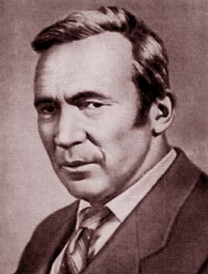
Andrey Kolmogorov (1903--1987) from Moscow University (Russia), as a student at the age of 19, in his very first scientific work, constructed an example of an absolutely integrable function whose Fourier series diverges almost everywhere (later improved to diverge everywhere).
This makes 𝔏¹-case even more pathological.
Example 2:
Kolmogorov's proof consists of two parts. First, we show that if there exists a sequence {φn} of sufficiently pathological integrable functions, then a suitable infinite linear combination of them is a desired function. After that, we construct those functions φn.
What do we want from the functions φn? First of all, they should be close to having a divergent Fourier series; the function φn should have a Fourier partial sum that is large as a function of n in a subset of [0,1] with large measure (this measure should approach 1). Moreover, we want some control over their linear combinations, so we require that the functions are nonnegative and that the 𝔏¹-norms are constant. We formulate these requirements more precisely.
Lemma:
There exists a sequence {φn} of integrable functions on [0,1] such that
φn ≥ 0 and ∥φn∥1 = 2.
The Fourier partial sums of φn are uniformly bounded.
There exists a sequence {Mn} tending to infinity such that the qnth Fourier partial sum of φn has absolute value greater than Mn in a set En ⊂ [0,1], where m(En) → 1 as n → ∞ (m(⋅) is the Lebesgue measure and qn is just a suitable number).
Assume for now that this has been proved. We apply this to prove
Theorem of Kolmogorov:
There exists an 𝔏¹-function whose Fourier series diverges almost everywhere.
where the nk are chosen suitably, and show that this function has an almost everywhere divergent Fourier series. Choose
n₁ < n₂ < n₃ < ⋯ inductively in the following way.
\( \displaystyle M_{n_{k}} \ge 4^k . \)
All the Fourier partial sums of \( \displaystyle \varphi_{n_i} , \) i < k are bounded by \( \displaystyle \frac{1}{2}\,\sqrt{M_{n_k}} . \) in absolute value.
We have \( \displaystyle \frac{1}{2}\,\sqrt{M_{n_k}} \ge q_n \) for all i < k.
Clearly this can be done by taking nk to be very large in terms of n₁, n₂, … , nk-1.
Now
This is allowed since a series with nonnegative terms can be integrated termwise. We take N = qnr for some r, and x ∈ Enr. Then by (iii), the rth term in the previous sum is at least
\( \displaystyle \sqrt{M_{n_r}} \) in absolute value. The sum of the terms with k<r can be estimated as follows.
We conclude that for any r, the function Φ(x) has a Fourier partial sum that is larger in absolute value than \( \displaystyle \frac{1}{2}\, M_r -6 \) in the set \( \displaystyle E_{n_r} . \) If E = lim suprEnr (the set of those x belonging to infinitely many Enr), then E has measure 1 and for x ∈ E the Fourier partial sums of Φ at x are unbounded. ■
Proof of Lemma:
We are going to choose a fast growing sequence of integers m₁, m₂, …. We set m₁ = n, and define the mi inductively. When mk has been defined for some 1≤k≤n, let
\( \displaystyle \varphi_n (x) = \frac{m_k^2}{n} \)
for x on the interval \( \displaystyle I_k = \left( \frac{2k}{2n+1} - \frac{1}{m_k^2} , \frac{2k}{2n+1} + \frac{1}{m_k^2} \right) . \) Outside these intervals, set φn(x) = 0. Then φn(x) ≥ 0 trivially, and the integral of φn is 2, as the length of Ik is 2/m2k. Hence it remains to prove (iii).
The Nth Fourier partial sum is expressed through Dirichlet's kernel:
Such a number mk exists since the integral converges to 0 as mk → ∞ by the Riemann-Lebesgue lemma (notice that t and x belong to different intervals, so there is no problem with integrability). In particular, we may choose 2mk+1 to be divisible by 2n+1.
We have now defined the sequence {mk}, and hence φn for all n. In particular, the integral producing the partial sum, taken over ⋃i<kIi, is by construction less than 1 in absolute value. If we show that the corresponding integral over ⋃i<kIi is large in a set En whose measure tends to 1, we are done.
Let r≥k, x ∈ Jk, and write the mkth partial sum integral over Ir as
The first integrand is just the integral of a constant, while the second integrand, the difference of the Dirichlet kernels is by the mean value theorem at most
where the constant in the big O is at most 8π. Since
\( \displaystyle \left\vert \frac{2r}{2n+1} -x \right\vert \le \frac{2}{n^2} , \) we have by sin y ≥ 2/(πy) for y ∈ [0, π/2], the inequality
Denote this set by En. Since the measure of ⋃k>n−√nJk is trivially bounded by
\( \displaystyle \sqrt{n} \cdot \left( \frac{1}{2n+1} + \frac{4}{n^2} \right) , \)
the measure of the points not belonging to any Jk with
\( \displaystyle k < n - \sqrt{n} \) is
\( \displaystyle O \left( \frac{1}{\sqrt{n}} \right) . \)
On the other hand, for any \( k \le n- \sqrt{n} , \) the measure of x ∈ Jk not satisfying the desired inequality is not greater than
\( \displaystyle \frac{4}{n\pi \sqrt{\log n}} , \)
because if the integer part of \( \displaystyle \left( 2 m_k + 1 \right) \left\vert \frac{2k}{2n+1} - x \right\vert \) is fixed, the measure of such points is at most
\( \displaystyle \frac{4}{\pi \sqrt{\log n} \left( 2 m_k +1 \right)} , \) and the number of possible integer parts is at most
\( \frac{2 m_k +1}{n} . \) We conclude that the measure of x∈[0,1] that do not satisfy the inequality is
\( \displaystyle O \left( \frac{1}{\sqrt{\log n}} \right) , \) so m(En)→1 as n→∞. The proof of the Lemma is now finished, and this also completes the proof of the Theorem. ■
Kolmogorov's example actually gives a stronger divergence result for free:
Theorem:
There is an 𝔏¹-function whose Fourier series diverges in measure almost everywhere.
Proof: Consider the function Φ(x) again. If its partial sums SN(Φ; x) converged in measure in some set F, then every subsequence would have a pointwise almost everywhere in F convergent sub-subsequence (This is well-known). In particular, Sqnk(Φ; x) would have an almost everywhere in F converging subsequence. However, it is unbounded almost everywhere, and this is a contradiction. ■
End of Kolmogorov Example
Andrei Kolmogorov
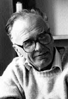
Lennart Carleson
A Swedish mathematician Lennart Axel Edvard Carleson (born 1928)
managed to prove in 1966 what was an authentic surprise for everybody: Luzin’s conjecture is true.
From that moment, the fact that the Fourier series of a function in 𝔏²([−ℓ, ℓ]) converges almost everywhere (except possibly on a set of “measure 0”) was known as Carleson’s theorem. The next year, Richard Hunt extended the almost everywhere convergence to 𝔏p([−π,π]) for 1< p<∞.
In 1966, Kahane and Katznelson complemented nicely Carleson's result by strengthening his claim: For any set E⊂(0,1) of measure zero, there exits a function whose Fourier series diverges on E.
The aim of this section is the proof of the following theorem.
Theorem (Carleson, 1966):
Suppose f is a square integrable function (in either the Riemann or Lebesgue sense) on a finite interval of length T. Then
where SN(f; x) is a partial Fourier sum of order N.
Of course, pointwise convergence is an important issue for Fourier series; however, we discuss this topic in the following section and
Cesàro summation in the next section.
Fourier series of a function f(x) can be considered as its restoration from the ordered discrete list (sequence) of its Fourier coefficients that we denote as | f ≫.
Since synthesizing a function from its Fourier series (or more precisely, from the list of its Fourier coefficients) is, generally speaking, an ill-posed problem, we cannot expect that finite partial Fourier sums always converge to the genius function. As it is shown in the following section, a pointwise convergence of Fourier series is a very delicate matter. Usually, ill-posed problems require some sort of regularization, and correspondingly Fourier series expansions were analyzed deeply and several regularizations are known.
The proof of Carleson was difficult to understand. Charles Fefferman proved Carleson’s theorem again in 1973. His methods were distinct to those of Carleson, but again difficult to follow. Later, in the context of their work in multilinear harmonic analysis, Lacey and Thiele came up with a quite short and relatively easy to understand proof for the 𝔏² theorem that is to some extent a descendant of Fefferman's proof. They also wrote an expository article describing this and a number of related results.
Note that between the space 𝔏¹([−ℓ, ℓ]) and the spaces 𝔏p[−ℓ, ℓ] ⊂ 𝔏¹[−ℓ, ℓ] for any p > 1 we have several function spaces on
which we can check convergence or divergence of Fourier series. Until now, we know that:
Essentially, the biggest space in which the convergence of the Fourier series of any
function has been proven is, as done by the Russian mathematician N.Yu. Antonov in 1996,
where log+ denotes the positive part of the logarithm.
Essentially, the smallest space in which it has been proven that there exists a function
whose Fourier series diverges is, as proven by Sergei Vladimirovich Konyagin in 2000,
We know so far that the biggest space in which convergence can be granted is somewhere between the Antonov space and the Konyagin one, but such space has not been found yet.
We now begin our study of Fourier analysis with the precise definition of
the Fourier series of a function. It is a custom to consider real-valued functions on a symmetric interval of length T = 2ℓ. Then for every Lebesgue interable function f : [−ℓ, ℓ] ↦ ℝ, we assign Fourier discretization list:
\[
𝔉: f(x) \mapsto |\, f \gg ,
\]
where | f ≫ is an infinite ordered discrete set (or sequence) of so called Fourier coefficients:
Note that there is no universal notation for complex conjugate numbers: mathematicians use overline, but physicists utilize asterisk. Hence, in order to please or confuse everyone, we use both notations.
Sometimes, exponential Fourier coefficients are defined slightly different; we identify such coefficients by calling them as
East Coast:
For existence of Fourier coefficients, function f must be integrable over the interval [−ℓ, ℓ] because the coefficient \( \frac{a_0}{2} = \hat{f}(0) = \frac{1}{2\ell} \,\int_{-\ell}^{+\ell} f(x)\,{\text d} x \) exists for f ∈ 𝔏¹. Hence, the Fourier coefficients should be considered for integrable functions.
The set of Riemann integrable functions is the most general class of functions we will be concerned with.
Such functions are bounded, but may have infinitely many discontinuities of measure zero. However, Fourier coefficients in equations \eqref{EqMode.1} and (2) exist for more wider class of functions---Lebesgue integrable functions. The latter set is denoted by 𝔏¹[−ℓ, ℓ].
Now we go into an opposite direction: for a given discrete data
\( \displaystyle 𝔉(f) = |\,f \gg , \) we want to recover function f. Hence, we need to solve the inverse problem
where 𝔉† stands for ill-posed (pseudo-) inverse of linear operator 𝔉 when its inverse 𝔉−1 is not available. Actually, this inverse problem includes two distinct problems: for a given discrete data | · ≫, determine function f that generates the discrete list. Actually, this inveerse problem asks to determine a function f whose finite replica | ≫N is close to the given one because we cannot handle infinte list.
Another inverse problem consists of synthetization of function f (analog signal) from its Fourier coefficients (again, finite subset). In this tutorial, we concentrate our attention of recovering function f from known discrete data | f ≫ written in
either in exponential (complex) form (1) or trigonometric form (2). It turns out that the solution of the latter is known as
the Fourier series; it can be written in either exponential (complex) form
Here T = 2ℓ is the length of the symmetric interval where function f is defined and x ∈ [−ℓ, ℓ] is a real variable.
As usual, j denotes the unit (imaginary) vector on complex plane ℂ, so j² = −1.
Here «P.V.» abbreviates the Cauchy principal value, which is a regularization of the infinite summation (obviously, the infinite summation is impossible to accomplish).
When function f is not smooth or when Fourier coefficients \eqref{EqMode.1} or (2) approach zero slowly, the Fourier series converges conditionally. Evaluation of such series becomes an ill-posed problem, so a natural definition of two-sided infinite series (that you learn in calculus)
does not work. If you set M = N in the formula above, it will provide you the Cauchy principal value regularization. Actually summing infinite terms is obviously an impossible task. What we can do is only to add up more and more
terms and continue to do so, but without hope of ever coming to an
end. So in practice, we operate with finite sums evaluated according to the Cauchy principal value; however, we can never close the gap between infinite sum and its truncated approximation completely.
The equal sign in the expression \( f(x) \,=\, \sum_{n=-\infty}^{\infty} \hat{f}(n)\, e^{n{\bf j} \pi x/\ell} . \) undoubtedly originates from a time when the true
nature of a limit process was not clearly understood and a limit was
considered as something obtained rather than something in the state
of becoming. Hence, the "equal" sign has to be understood as
"as nearly equal as we wish."
In addition, Fourier series may or may not converge, and if it converges, we don't know whether its sum S[f] is equal to f(x),
we use a tilde (∼) instead of equal symbol (=) simply to manifest the fact that the Fourier coefficients \( \hat{f}(n) \) are evaluated according to Eq.\eqref{EqMode.1} and the Fourier series S[f] is the limit of its partial sums; similarly, the coefficients in «identity» \eqref{EqMode.4} are evaluated according to Euler--Fourier formulas (2). Therefore, the right-hand sides of Eqs.\eqref{EqMode.3} or \eqref{EqMode.4} provide a formal expression that we denote by S[f].
We use notation S[f] for symbolic manipulations---a powerful
formalism in contemporary applied mathematics that helps us to tackle even difficult physical problems. S[f] symbolizes the limiting process that sits inside this notation. It is similar to the definition of π:
You enjoy elegance of the formal
manipulations with π, but you
have no way of defining this number by a finite construction. Another example of finite approximation of actual limiting process you observe when plotting a circle on your screen or printout. Actually, a computer provides you only polygon approximation (not differentiable) to the circumference (which is a smooth function). Therefore, S[f] symbolizes that you can approximate the genius function f with any accuracy you want subject the Fourier series converges to it.
For any real x, the finite sum
\[
F_N (x) = \frac{a_0}{2} + \sum_{k=1}^{N} \left[ a_k \cos \left( \frac{\pi}{\ell}\, k x \right) + b_k \sin \left(
\frac{\pi}{\ell}\,k x \right) \right]
\]
If coefficients αn and 𝑎k, bk are evaluated according to the Euler--Fourier formulas \eqref{EqMode.1} and (2), respectively, then trigonometric polynomial FN is called N-th Fourier partial sum and it is denoted by SN(f; x) or simple SN(f).
In calculus, you learn that an infinite series \( \sum_{k\ge 0} a_k \) converges (or is convergent) to S if the sequence of partial sums \( S_n = \sum_{k= 0}^n a_k \) tends to S as n → ∞. In case of Fourier series, elements of series depend on real parameter x ∈ [−ℓ, ℓ], and we come to definition of its partial sums.
Theorem 2:
For any real-valued function f : [−ℓ, ℓ] → ℝ and any positive integer N ∈ ℕ = { 0, 1, 2, … }, its N-th partial Fourier exponential sum
\begin{equation} \label{EqFourier.6}
S_N (f;x) = \frac{1}{2}\,a_0 + \sum_{k=1}^N \left[ a_k \cos \left( \frac{\pi}{\ell}\, k x \right) + b_k \sin \left( \frac{\pi}{\ell}\, k x \right) \right]
\end{equation}
are the same; here coefficients 𝑎k, bk and \( \displaystyle \hat{f}(n) \) are determined by the Euler--Fouier formulas (2) and \eqref{EqMode.1}, respectively. Moreover, the N-th partial Fourier sum is expressed in an integral form, known as a convolution, which is denoted by star:
Theorem 2 was proved in section of this tutorial. These formulas show that partial Fourier sums are independent of the way you define them, either exponential (5) or trigonometric (6). Also the Dirichlet kernel is also the same on West coast or East one.
Example 3:
We check Dirichlet's kernel for some small values of n. If n = 2, we have
approach a limit when N → ∞.
Therefore, we need to introduce a criteria for their convergence. So we start with the general definition of series convergence. Besides this classical definition of series convergence (that you learn in calculus), there are known several other generalizations of this convergence. One of them is
considered in Cesàro section).
To define a Fourier series, we need two things. First, we must have a class of expandable (admissible) functions for which Fourier series makes sense (because Fourier series does not exist for arbitrary function). Second, we need to identify a metric or distance between elements in the function space. In this course, we consider only metrics that are generated by norms. So we consider the following function spaces and corresponding convergent criteria.
The supremum (abbreviated as sup) in the norm definition \( \|f(x) \|_{\infty} \) means a smallest number K such that |f(x)| ≤ K for almost all x. If functions involved are continuous, supremum can be replaced with maximum.
That is, the overall “distance” between the function f(x) and the partial Fourier sums SN(f; x) converges
to zero. Notice that the endpoints of the interval are included in the definition.
This infinite norm is usually applied to the set of continuous functions defined either on closed interval [−ℓ, ℓ] or on one-dimensional torus 𝕋 (which is a unit circle). The corresponding function spaces are denoted by ℭ[−ℓ, ℓ] or ℭ(𝕋), respectively.
The set of all (measurable) unctions having finite mean square norm is usually denoted by 𝔏²([−ℓ, ℓ]) (notations L² and L2 are also in use). Actually, this norm is generated by the inner product:
\[
\langle f \,\vert\, g \rangle = \int_{-\ell}^{+\ell} f(x)^{\ast} g(x)\,{\text d} x = \langle f \,,\, g \rangle ,
\]
where asterisk stands to complex conjugate.
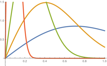
Example 4:
Consider the sequence of functions
\( \displaystyle f_n (x) = 2nx\,e^{-n\, x^2} , \quad n=1,2,\ldots , \) on interval [0, 1]. Since the exponential function majorates any polynomial, the given sequence converges pointwise to zero. However,
This example illustrates that the pointwise limit of a sequence of functions
does not always inherit the properties of the sequence functions.
Plot of four terms in the sequence for n = 1, 3, 10, 100.
Mathematica code
End of Example 4
Two functions from either 𝔏¹([−ℓ, ℓ]) or 𝔏²([−ℓ, ℓ]) will be identical if they differ only on a set of measure 0; especially, f is identifies with the zero function if f(x) = 0 almost everywhere. This will allow you to claim ∥ f ∥ = 0 if and only if f(x) ≡ 0.
Technically, as a normed linear space, the 𝔏p space consists of equivalence classes of such functions, where two functions are equivalent if and only if they differ on a set of measure zero. This is because a function that is zero only almost everywhere, under this definition, will still have norm zero. However, we can usually refer to an element of an 𝔏p space as a function instead of an equivalence class of functions without much trouble. Also, to be complete, integration in the definition of the norm should be understood in Lebesgue sense rather than in Riemann one.
The most important in practice is the pointwise convergence of Fourier series, which is
discussed in the next section. The uniform convergence is the strongest of
the other three: it
implies pointwise convergence as well as 𝔏p-convergence for any p ≥ 1.
However, pointwise convergence is weakly related to the mean convergence because discrete values of a function do not effect its integral value.
Example 5:
Let us consider a sequence of functions on the interval [0, 1],
This sequence converges to 0 for every x ∈ [0, 1]. However,
\[
\int_0^1 \left\vert f_n (x) \right\vert^2 {\text d} x = \int_0^{1/n} \left\vert f_n (x) \right\vert^2 {\text d} x = n^2 \times \frac{1}{n} = n .
\]
So fn does not converge to zero function in 𝔏²[0, 1].
End of Example 5
Let X be a normed linear space, and let xn, x ∈ X. We say that xn converges strongly, or converges in norm to x, and write
xn → x, if
\[
\lim_{n\to\infty} \| x_n - x \| = 0.
\]
Despite these two examples, there is a relation between mean square mode of convergence and pointwise convergence.
Theorem 3:
If sequence of square integrable functions fn strongly
converges to f ∈ 𝔏²([−ℓ, ℓ]), then there exists subsequence n₁ < n₂ < n₃ < ⋯ ↑ ∞ so that fnk converges to f pointwise almost everywhere.
Because limn↑ ∞ ∥ fn − f ∥ = 0, we can pick up n₁ < n₂ < n₃ < ⋯ ↑ ∞ so that
\[
\| f_{n_k} - f \|^2 \le 2^{-k} \qquad \mbox{for} \quad k = 1,2,3,\ldots .
\]
The Euler--Fourier formulas (1) or (2) show that the Fourier coefficients are evaluated
as integrals over the whole interval where a function is defined (it is
convenient to integrate over symmetrical interval [−ℓ ,ℓ] because the function is extended periodically by its Fourier series). Therefore,
these coefficients are influenced by the behavior of the function over the
interval. This is completely different from Taylor series where coefficients
are determined by the infinitesimal behavior of the function at the center of
expansion because they are calculated as derivatives at the point. On the
other hand, integral does not depend on the value of integrand function at
discrete number of points. So it is expected that we cannot restore the value
of the function at particular point from its Fourier series---Fourier
coefficients do not contain this information. In contrast, Taylor series
provide such information and pointwise or uniform convergence is appropriate
for them. Fourier series are based on another convergence that is called
𝔏² (square mean), and it is completely different type of
convergence. The advantage of this convergence is obvious: discontinuous functions could be expanded into Fourier series but not into Taylor series.
Example 6:
We consider three functions on interval (−ℓ, ℓ):
\[
\| f \| = \sqrt{\langle f, f \rangle} = \left( \int_{-\ell}^{\ell} \left\vert f(x) \right\vert^2 {\text d} x \right)^{1/2} = \| f \|_2 .
\]
A sequence { ϕn } of elements in a Hilbert space is said to be orthogonal if ⟨ ϕn, ϕk ⟩ = 0 for n ≠ k.
A sequence { en } of elements in a Hilbert space
is called an orthonormal sequence, n = 1, 2, . . . , if 〈en, ek〉 = 0 for n ≠ k
and 〈en, en〉 = ‖en‖² = 1.
Every orthogonal sequence can be transferred into the orthonormal sequence upon division every element by its norm: en = ϕn/‖ϕn‖.
Let { en }n∈ℤ be the orthonormal sequence of functions on interval [−ℓ, ℓ]:
Lemma (Best approximation):
For a squre integrable on interval [−ℓ. ℓ] function
f∈𝔏²([−ℓ, ℓ]) and orthonormal set of functions { en }, the mean square erroe E, defined by
\[
E = \left\| f - \sum_{k=0}^N c_k e_k \right\|^2
\]
is minimized when coefficients ck are the Fourier coefficients of function f:
where \( \displaystyle b_n = a_n - \hat{f}(n) . \)
This lemma has a clear geometric interpretation. It says that the
trigonometric polynomial of degree at most N that is closest to f in the mean square norm is the partial Fourier sum SN(f).
Theorem 4:
Let f be a square-integrable function, f ∈ 𝔏²([−ℓ, ℓ]). A trigonometric polynomial of degree N that best approximates f in the norm ||·||2 is the Nth Fourier sum \eqref{EqMode.4} of f.
The first two terms of the last expression do not depend on p(x), whereas the last one does. Since all the terms in the last term are positive, the only choice to minimize it is to set ck = 𝑎k and dk = bk for every k
Theorem 5 (Bessel's inequality):
Suppose that f(x) is a square integrable function on the interval [𝑎, b]. Let 𝑎k, bk and \( \hat{f}(n) \) be the Fourier coefficients defined by Eq.(2) and Eq.(1), respectively. Then
Since the left-hand side is positive (at least not negative) we obtain the required inequality when N → ∞,
Parseval Identity
Actually, Bessel's inequality can be improved and converted into identity, named after Marc-Antoine Parseval (1755--1836) that expresses the energy of a signal in time-domain in terms of the average energy in its frequency components. In 1799, he stated the following theorem, but did not prove (claiming it to be self-evident). It is also known as Rayleigh's energy theorem, or Rayleigh's identity, after John William Strutt, Lord Rayleigh. [Rayleigh, J.W.S. (1889) "On the character of the complete radiation at a given temperature," "Philosophical Magazine", vol. 27, pages 460-469.]
Although the term "Parseval's theorem" is often used in applications, the most general form of this property is more properly called the Plancherel theorem.
Parseval des Chênes, Marc-Antoine "Mémoire sur les séries et sur l'intégration complète d'une équation aux differences partielle linéaire du second ordre, à coefficiens constans" presented before the Académie des Sciences (Paris) on 5 April 1799. This article was published in "Mémoires présentés à l’Institut des Sciences, Lettres et Arts, par divers savans, et lus dans ses assemblées. Sciences, mathématiques et physiques. (Savans étrangers.)", vol. 1, pages 638-648 (1806).
Plancherel, Michel (1910) "Contribution a l'etude de la representation d'une fonction arbitraire par les integrales définies," "Rendiconti del Circolo Matematico di Palermo", vol. 30, pages 298-335.
where the Fourier coefficients \( \hat{f}(n) \) and 𝑎k, bk are defined by equations (1) and (2), respectively.
Parseval's identity is a fundamental result on the summability of the Fourier series of a function. It actually establishes completeness of the set of eigenfunctions of the Sturm--Liouville operator \( H(\hat{p}) = - \texttt{D}^2 = - {\text d}^2 /{\text d} x^2 . \)
For a real-valued function f ∈ 𝔏²([−ℓ, ℓ]), the Parseval identity can be written as
There is another theorem that is closed related to the Parseval theorem. It was proved independently by Frigyes Riesz (Sur les systèmes orthogonaux de fonctions et l’équation de Fredholm, Comptes Rendus de l'Académie des sciences, 1907,
144, pp. 734-736) and Ernst Sigismund Fischer (Sur la convergence en moyenne, Comptes rendus de l'Académie des sciences, 144, pp. 1022–1024).
Later in 1910, F. Riesz published a detailed exposition of his results in Hungarian.
Riesz--Fischer Theorem:
Let { en } be an orthonormal sequence in 𝔏²([𝑎, b]). Given a sequence {cn} of scalars such that \( \sum_{n=-\infty}^{\infty} \left\vert c_n \right\vert^2 < \infty , \) there exists an f in 𝔏²([𝑎, b]) for which
Example 8:
Consider an integrable function on [0, 1] with infinitely
many discontinuities is given by
\[
f(x) = \begin{cases}
1 , & \ \mbox{ if } \ 1/\left( n+1 \right) < x \le 1/n \ \mbox{ and $n$ is odd}, \\
0, & \ \mbox{ if } \ 1/\left( n+1 \right) < x \le 1/n \ \mbox{ and $n$ is even}, \\
0, & \ \mbox{ if } \ x = 0.
\end{cases}
\]
The function f is discontinuous
when x = 1/n and at x = 0.
■
Since infinite sums of squares of Fourier coefficients converge, we immediately deduce that Riemann-Lebesgue lemma is valid for functions from
𝔏²([−ℓ, ℓ]):
The Euler--Fourier formulas, either complex (1) or trigonometric (2), define a sequence \( \left\{ \hat{f}(n) \right\}_{n\in\mathbb{Z}} \) of complex numbers or a sequence of pairs of real numbers {(𝑎k, bk}k∈ℕ, respectively. These sequences or infinite vectors can be considered as discretization of the analog signal defined by function f(x).
The Parseval identity tells us that that these sequences of numbers should belong to the complete space of sequences in its norm, denoted as ℓ²(ℤ) or ℓ²(ℕ²), that consist of all sequences for which
\[
\left\| \left\{ \hat{f}(n) \right\} \right\|_2 = \sum_{n=-\infty}^{\infty} \left\vert \hat{f}(n) \right\vert^2 < \infty \qquad\mbox{or} \qquad
\| \left\{ \left( a_k , b_k \right) \right\} \|_2 = \frac{1}{2}\,a_0^2 +
\sum_{k\ge 1} \left( a_k^2 + b_k^2 \right) < \infty ,
\]
respectively. Here ℤ = { 0, ±1, ±2, … } is the set of all integers and ℕ = { 0, 1, 2, … } is the set of all nonnegative integers.
However, not every sequence {αn}n∈ℤ from ℓ²(ℤ) defines a function \( \sum_{n\pm\mathbb{Z}} \alpha_n e^{{\bf j} n\omega x} , \quad \omega = \frac{\pi}{\ell} , \) that is square integrable in Riemann sense. It turns out that the Fourier series (3) defines a function that is Lebesgue square integrable.
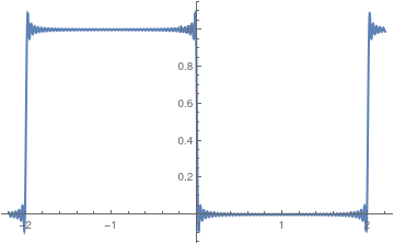
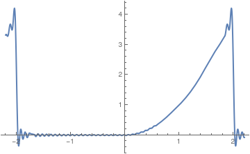
Example 9:
Let us consider a piecewise continuous function on interval [−π, π]:
Corollary:
If f(x) is a square integrable function (we abbreviate it as f∈𝔏²) then its Fourier coefficients tend to zero as n → ∞.
If we were to assume that the Fourier series of functions f converge to f in an appropriate sense, then we could infer that a function is uniquely determined by its Fourier coefficients. This would lead to the following statement: if f and g have the same Fourier coefficients, then f and g are necessarily equal. By taking the difference f − g, this proposition
can be reformulated for the zero function. As stated,
this assertion cannot be correct without reservation, since calculating
Fourier coefficients requires integration, and, for example,
any two functions which differ at finitely many points have the same
Fourier series.
Theorem 4:
Let f(x) be an integrable function (in the Lebesgue sense) on a symmetrical interval [−ℓ, ℓ]. If all its Fourier coefficients are zeroes, then f(x) = 0 whenever f is continuous at the
point x.
We prove Carleson Theorem for the case when ω = π/ℓ = 1 (that is, ℓ = π). In this case, the eigenfunctions \( \displaystyle e_n (x) = e^{{\bf j}nx} , \) n ∈ ℤ, foorm an orthonormal system in 𝔏²[−π, π]:
Let αn be Fourier coefficients of function
f ∈ 𝔏²[−π, π]:
\[
\alpha_n = \langle e_n \vert f \rangle = \int_{-\pi}^{\pi} e^{-{\bf j}nx} f(x)\,{\text d} x , \qquad n \in \mathbb{Z} .
\]
Then the orthonormal property of
the family { en } and the fact that αn = ⟨ en, f ⟩
imply that the difference \( \displaystyle f - \sum_{n=-N}^N \alpha_n e_n \)
is orthogonal to en for all |n| ≤ N. Therefore, we must
have
for any complex numbers bn. We draw two conclusions from this fact.
First, we can apply the Pythagorean theorem (∥x + y∥2 = ∥x∥2 + ∥y∥2 for orthogonal vectors x⊥y) to the decomposition
\[
f = f - \sum_{|n|\le N} \alpha_n e_n + \sum_{|n|\le N} \alpha_n e_n ,
\]
\[
\| f \|^2 = \| f - S_N (f; x) \|^2 +
\sum_{|n|\le N} \left\vert \alpha_n \right\vert^2 .
\]
To finish the proof of Carleson's theorem, we apply the best approximation lemma as well as the important fact that trigonometric
polynomials are dense in the space of continuous functions.
Suppose that f is continuous on interval [−π, π]. Then, given ϵ > 0, there
exists a trigonometric polynomial P, say
of degree M, such that
In particular, taking squares and integrating this inequality yields ∥f − P∥ < ϵ, and by the best approximation lemma we conclude that
\[
\left\| f - S_N (f) \right\| < \epsilon \qquad \mbox{whenever } N \ge M. .
\]
This proves Carleson's theorem when f is continuous.
If f is merely integrable, we can no longer approximate f uniformly
by trigonometric polynomials. Instead, we apply the
following approximation Lemma
Approximation Lemma:
Suppose f ∈ 𝔏¹[𝑎, b] is integrable on [𝑎, b] and bounded by K.
Then there exists a sequence { fn }n≥1
of continuous functions on [𝑎, b] so that
\[
\sup_{x\in [a, b]} \left\vert f_n (x) \right\vert \leqslant K \qquad \mbox{for all } n =1, 2, 3, \ldots ,
\]
\[
\int_{-\pi}^{\pi} \left\vert g (x) - f(x) \right\vert {\text d} x < \epsilon^2 .
\]
Then we get
\begin{align*}
\| f - g \|^2 &= \int_{-\pi}^{\pi} \left\vert g (x) - f(x) \right\vert^2 {\text d} x
\\
&= \int_{-\pi}^{\pi} \left\vert g (x) - f(x) \right\vert \, \left\vert g (x) - f(x) \right\vert {\text d} x
\\
&\le 2K \int_{-\pi}^{\pi} \left\vert g (x) - f(x) \right\vert {\text d} x
\\
&\le C\,\epsilon^2 .
\end{align*}
Hence, we may approximate g by a trigonometric polynomial P so that ∥g − P∥ ≤ ϵ. Then ∥f − P∥ ≤ cϵ, and we may again conclude by applying the best approximation lemma. This completes the proof that the
partial sums of the Fourier series of f converge to f in the mean square norm.
This definition can be specified for our two Banach spaces, 𝔏¹[𝑎, b] and 𝔏²[𝑎, b].
A sequence of points {xn} in a Hilbert space ℌ is said to converge weakly to a point x in ℌ if
\[
\langle y\,\vert\, x_n \rangle \, \to \,\langle y\,\vert\, x \rangle \qquad \mbox{as} \quad n \to \infty
\]
for all y in ℌ. Here ⟨ ⋅|⋅ ⟩ or ⟨ ⋅,⋅ ⟩ is understood to be the inner product in the Hilbert space.
A sequence of points {xn} in a Banach space 𝔏¹[−ℓ, ℓ] converges weakly to x ∈ 𝔏¹
if the sequence of scalars
\[
\int_{-\ell}^{\ell} f(t)\,x_n (t)\,{\text d} t \,\to \, \int_{-\ell}^{\ell} f(t)\,x (t)\,{\text d} t \qquad \mbox{as} \quad n \to \infty
\]
for all bounded functions f ∈ 𝔏∞[−ℓ, ℓ]. When a sequence {xn} converges to x weakly, we abbreviate it as
xn ⇀ x.
In particular, a sequence {xn}n∈ℕ of elements xn = [xn,0, xn,1, …] ∈ ℓ² converges weakly to x if and only if the following two conditions hold:
there exists a positive constant C such that |xn,k| ≤ C;
for each k, xn,k → xk.
We need weaker convergence than defined above weak convergence. This new definition requires usage of dual space X* that consists of all continuous linear functionals over the normed space X.
Let X be a normed linear space. A sequence of functionals { fn } ⊆ X* is weak* or weak-star
convergent to f ∈ X* if sequence of scalars { fn(x) } converges to f(x) for all x ∈ X.
A weak-star convergence is denoted by xn ⇁ x.
The most famous application of the weak-star convergence provides the following lemma. It considers a trigonometric polynomial as a functional on 𝔏¹.
This sequence does not converge in ℓ² because it is not Cauchy sequence: \( \displaystyle \| \delta_n - \delta_m \|_2 = \sqrt{2} \) for n ≠ m. However, the sequence converges weakly to 0. Indeed, for g ∈ ℓ², we have
where we represent g as a vector [g(1), g(2), g(3), … ]. Since the general term of this vector tends to zero, we conclude that that the sequence {δn} converges weakly to zero.
However, this sequence {δn} of standard basis does not converge in ℓ¹. To prove this,we define the linear functional φ on ℓ¹ by
So the sequence {φ(δn)} is not Cauchy in ℝ; hence, not convergent.
Thus the standard basis of ℓ¹ does not converge weakly.
Uniqueness Theorem:
If {xn} converges weakly to both x and y, then x = y.
Suppose that {xn} converges weakly to both x and y, then for every functional T, the sequence of scalars
{T xn} converges to both T x and T y. However, this is impossible because any sequence of scalars has at most only one limit value.
Radon--Riesz Theorem:
Suppose {fn} converges weakly to f
in 𝔏²[−ℓ, ℓ]. Then {fn} converges to f in 𝔏²[−ℓ, ℓ] if and only if
\( \displaystyle \lim_{n\to\infty} \| f_n \| = \| f \|_2 . \)
The theorem was first proved in 1913 by the Austrian mathematician Johann Radon (1887--1956).
A proof of the Radon--Riesz Theorem can be found in Royden and Fitzpatrick's book. The general proof for arbitrary p ≥ 1 is presented in
Riesz and Sz.-Nagy’s
Functional Analysis, London: Blackie & Son Limited (1956) (reprinted by Dover
Publishing in 1990). It is also on the web:
http://faculty.etsu.edu/gardnerr/5210/notes/Radon-Riesz.pdf.
Example 11:
Let us consider the following sequence of points from ℓ²:
Indeed, all entries in xn,k are bounded by 1 and every its entry tends to zero as n → 0. However, this sequence does not converge to x uniformly because
\[
\| x_n - x \|_2 = 1 .
\]
On the other hand, if we slightly modify the sequence above by placing on n-th position 1/n instead of 1, we get the sequence
Then this sequence converges strongly to x because
\[
\| y_n - x \|_2 = \frac{1}{n} \to 0 \qquad \mbox{as}\quad n \to \infty .
\]
From the Radon-Riesz theorem, we immediately derive that every function f ∈ ℓ² has a weak convergent Fourier series S[f]. Since 𝔏²[−ℓ, ℓ] ⊂ 𝔏¹[−ℓ, ℓ], we have another result.
Schur’s Lemma:
In ℓ¹, if a sequence {fn} converges weakly to f, fn ⇀ f, then this sequence strongly converges to f.
Proof of Schur's property can be found in Megginson's book, section 2.5.24.
Although weak and strong convergences are equivalent in ℓ¹, they are different in 𝔏¹[𝑎, b]. For example, the sequence of eigenfunctions \( \displaystyle \phi_n = e^{{\bf j} nx} \) converges to zero weakly, but does not converge in 𝔏¹ because their norms are constants:
Antonov, N.Yu., Convergence of Fourier series, East Journal on Approximations, Volume 2, Number 2, 1996, pp. 187–196. (Proceedings of the XX Workshop on Function Theory, Moscow, 1995).
du Bois-Reymond, P., Ueber die fourierschen reihen,
Königliche Gesellschaft der Wissenschaften zu Göttingen,
1873, Vol. 21, pp. 571--582.
Hunt, R.A., On the convergence of Fourier series,
Proc. Conf. Orthogonal Expansions and their Continuous Analogues, Southern Illinois Univ. Press (1968) pp. 234–255.
Kahane, J. and Katznelson, Y., Sur les ensembles de divergence des séries trigonométriques, Studia Mathematica, 1966,
Volume: 26, Issue: 3, pages 307-313.
Konyagin, S.V., On divergence of trigonometric Fourier series, Comptes Rendus de l'Académie des Sciences - Series I - Mathematics, 1999, Vol. 329, pp.693--697.
Konyagin, S.V., On everywhere divergence of trigonometric Fourier series, Sb. Math. 191 (1), 97–120 (2000) [transl. from Математический сборник, 2000, 191, No. 1, pp. 103–126].
Körner, T.W., Fourier Analysis, Cambridge University Press, Great Britain, 1989.
Lacey, M. and Thiele, C., (2000), "A proof of boundedness of the Carleson operator", Mathematical Research Letters, 2000, Vol. 7 (4), pp. 361–370.
Lacey, M. and Thiele, C., Carleson's theorem: proof, complements, variations, Publicacions Matemàtiques, 2004, Vol. 48 (2), pp. 251–307
Luzin, N.N., The integral and trigonometric series (In Russian), 1915, Moscow-Leningrad (Thesis; also: Collected Works, Vol. 1, Moscow, 1953, pp. 48–212).
Megginson, R.E., An Introduction to Banach Space Theory 1998, Springer.
Ul'yanov, P.L., Kolmogorov and divergent Fourier series, Uspekhi Mat Nauk, 1983, Vol. 38, No. 4, 51--90; Russian math Surveys, 1983, 38, No. 4, pp. 57--100.
Return to Mathematica page for APMA0360
Return to the main page (APMA0360)
Return to the Part 1 Basic Concept
Return to the Part 2 Fourier Series
Return to the Part 3 Integral Transformations
Return to the Part 4 Parabolic Equations
Return to the Part 5 Hyperbolic Equations
Return to the Part 6 Elliptic Equations
Return to the Part 7 Numerical Methods