Linear equations from electrical circuits
Developing linear equations from electric circuits is based on two Kirchhoff's laws:- Kirchhoff's current law (KCL): at any node (junction) in an electrical circuit, the sum of currents flowing into that node is equal to the sum of currents flowing out of that node
- Kirchhoff's voltage law (KVL): the sum of the emfs in any closed loop is equal to the sum of the potential drops in that loop.
- when we travel around a loop of the circuit, the algebraic sum of the volts has to be equal to zero;
- always start at the battery.
Example:
Consider a simple circuit with two resistors depictured in the figure.
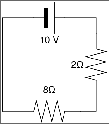
One loop circuit
To derive the equations that describe the given one loop circuit, we use the
following steps:
battery[l_: 1] := {gap[
l], {Rectangle[l {1/3, -(1/3)}, l {1/3 + 1/9, 1/3}],
Line[l {{2/3, -1/2}, {2/3, 1/2}}]}};
resistor[l_: 1, n_: 3] := Line[Table[{i l/(4 n), 1/3 Sin[i Pi/2]}, {i, 0, 4 n}]];
contact[l_: 1] := {gap[l], Map[{EdgeForm[Directive[Thick, Black]], FaceForm[White], Disk[#, l/30]} &, l {{1/3, 0}, {2/3, 0}}]};
Options[display] = {Frame -> True, FrameTicks -> None, PlotRange -> All, AspectRatio -> Automatic};
display[d_, opts : OptionsPattern[]] := Graphics[Style[d, Thick], Join[FilterRules[{opts}, Options[Graphics]], Options[display]]];
at[position_, angle_: 0][obj_] := GeometricTransformation[obj, Composition[TranslationTransform[position], RotationTransform[angle]]];
label[s_String, color_: RGBColor[.3, .5, .8]] := Text@Style[s, FontColor -> color, FontFamily -> "Times", FontSize -> Large];
display[{connect[{{0, -2}, {0, 1}, {1, 1}}], battery[] // at[{1, 1}], connect[{{2, 1}, {3, 1}, {3, 0}}], resistor[] // at[{3, 0}, 3 Pi/2], connect[{{3, -1}, {3, -2}, {2, -2}}], resistor[] // at[{1, -2}], connect[{{1, -2}, {0, -2}}], Text[Style["2\[CapitalOmega]", FontSize -> 30], {2.4, -0.5}], Text[Style["10 V", FontSize -> 30], {1.5, 0.3}], Text[Style["8\[CapitalOmega]", FontSize -> 30], {1.5, -1.3}]}]
- Start from the battery.
- The current flow from the battery is clockwise. Therefore, we start on the + side: 10 v.
- Traveling clockwise to the 2 Ω: 10 v + 2 i.
- Traveling clockwise once again to the 8 Ω:10 v + 2 i + 8 i = 0.
- We have completed our equation because we have only one loop, so there is a single equation for voltage v and current i.
Example:
Now we consider a two loop circuit.
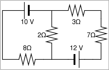
Two loop circuit
Since the above circuit consists of two loops, we derive equations between
voltage v and current i for each loop. For the first circuit, we
use the following steps:
label[s_String, color_: RGBColor[.3, .5, .8]] :=
Text@Style[s, FontColor -> color, FontFamily -> "Times",
FontSize -> Large];
display[{connect[{{1, -2}, {0, -2}, {0, 1}, {1, 1}}], battery[] // at[{2, 1}, Pi], connect[{{2, 1}, {3, 1}, {3, 0}}], resistor[] // at[{3, 0}, 3 Pi/2], connect[{{3, -1}, {3, -2}, {2, -2}}], resistor[] // at[{1, -2}], connect[{{3, 1}, {4, 1}}], resistor[] // at[{4, 1}], connect[{{5, 1}, {6, 1}, {6, 0}}], resistor[] // at[{6, 0}, 3 Pi/2], connect[{{6, -1}, {6, -2}, {5, -2}}], battery[] // at[{4, -2}], connect[{{3, -2}, {4, -2}}], Text[Style["2\[CapitalOmega]", FontSize -> 20], {2.4, -0.5}], Text[Style["7\[CapitalOmega]", FontSize -> 20], {5.4, -0.5}], Text[Style["3\[CapitalOmega]", FontSize -> 20], {4.5, 0.3}], Text[Style["10 V", FontSize -> 20], {1.5, 0.3}], Text[Style["8\[CapitalOmega]", FontSize -> 20], {1.5, -1.3}], Text[Style["12 V", FontSize -> 20], {4.5, -1.3}]}]
display[{connect[{{1, -2}, {0, -2}, {0, 1}, {1, 1}}], battery[] // at[{2, 1}, Pi], connect[{{2, 1}, {3, 1}, {3, 0}}], resistor[] // at[{3, 0}, 3 Pi/2], connect[{{3, -1}, {3, -2}, {2, -2}}], resistor[] // at[{1, -2}], connect[{{3, 1}, {4, 1}}], resistor[] // at[{4, 1}], connect[{{5, 1}, {6, 1}, {6, 0}}], resistor[] // at[{6, 0}, 3 Pi/2], connect[{{6, -1}, {6, -2}, {5, -2}}], battery[] // at[{4, -2}], connect[{{3, -2}, {4, -2}}], Text[Style["2\[CapitalOmega]", FontSize -> 20], {2.4, -0.5}], Text[Style["7\[CapitalOmega]", FontSize -> 20], {5.4, -0.5}], Text[Style["3\[CapitalOmega]", FontSize -> 20], {4.5, 0.3}], Text[Style["10 V", FontSize -> 20], {1.5, 0.3}], Text[Style["8\[CapitalOmega]", FontSize -> 20], {1.5, -1.3}], Text[Style["12 V", FontSize -> 20], {4.5, -1.3}]}]
- Starting from the battery our direction is going from the - to the + position, counter clockwise. Therefore, we have a positive volt number: 12 v.
-
Traveling to the 2 Ω, we notice that the 2 Ω is being shared by
both circuits. Once again, we calculate by using the circuit that we are in
subtracted by the other circuit:
\[ _ 12\,v + 2 \left( i_1 - i_2 \right) , \]where i1 and i2 are currents in every loop, respectively.
-
Continuing on to 3 Ω:
\[ 12\,v + 2 \left( i_2 - i_1 \right) + 3\, i_2 . \]
-
Finally we approach 7 Ω, completing our i2 equation:
\[ \begin{split} 12\,v + 2 \left( i_2 - i_1 \right) + 3\,i_2 + 7\,i_2 &= 0, \\ -2\,i_1 + 12\,i_2 &= -12\,v . \end{split} \]
\[
\begin{split}
10\,i_1 - 2\,i_2 &= 10 , \\
-2\,i_1 + 12\,i_2 &= -12 . \end{split}
\]
We can use Mathematica to create an augmented matrix, row reduce and
solve:
m = {{10, -2, 10}, {-2, 12, -12}} ;
MatrixForm [m]
\( \begin{pmatrix} 10&-2&10 \\ -2&12&-12 \end{pmatrix} \)
RowReduce [m]
{{1, 0, 24/29}, {0, 1, -(25/29)}}
Therefore, i1 = 24/29 and i2 = -25/29.
■