Examples of Circuits

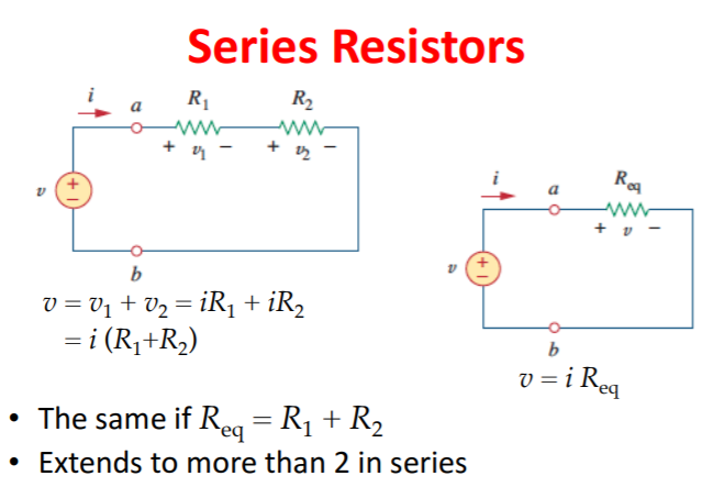
One of the basic fundamentals to simplifying and solving a circuit is to focus on multiple resistors that have connections with one another. Depending upon the configuration of the ladder network, the resistors in series can be added up to simplify the resistance in that certain region of the circuit.

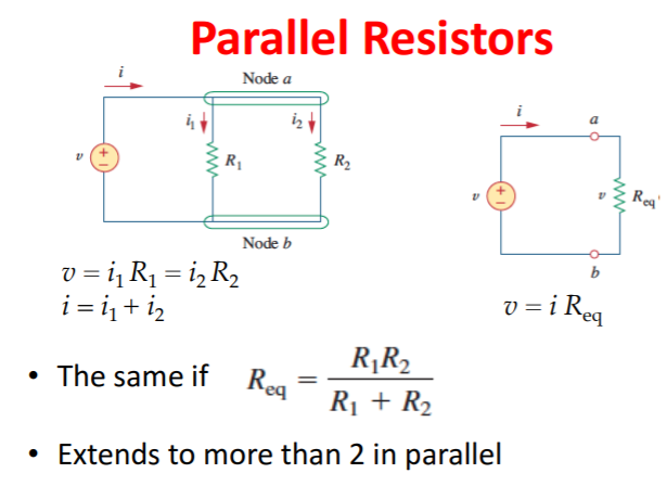
In addition, resistors in parallel can be combined by adding the inverse of all of the parallel resistances.

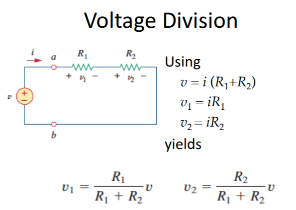
After the simplification of combining series and parallel resistors, there are operations in electrical engineering that can be used to solve for other elements in the circuit. For instance, having resistors in series enables the use of voltage division. Voltage division is a procedure that is used to solve for the voltage of a resistor (when that particular resistor is in series with another resistor in the circuit).

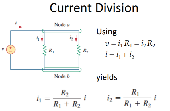
Moreover, resistors in parallel allows the use of an operation known as current division. Current division is a function that is used to solve for the current that passes through a resistor (when that particular resistor is connected in parallel with another resistor in the circuit).

The input voltage (v₁) and the input current (i₁) in an electrical circuit is set up in a matrix form that looks like \( \begin{bmatrix} v_1 \\ i_1 \end{bmatrix} . \) Meanwhile, the output voltage (v₂) and the output current (i₂) is set up in a column vector form that equates to \( \begin{bmatrix} v_2 \\ i_2 \end{bmatrix} . \) Taking a standard electrical circuit with a linear transformation is known as a transfer matrix, which is written as \( \begin{bmatrix} v_2 \\ i_2 \end{bmatrix} = {\bf A}\, \begin{bmatrix} v_1 \\ i_1 \end{bmatrix} . \)

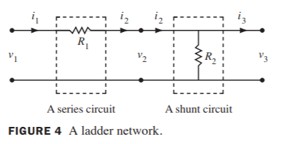
It is entirely possible that an electrical engineer could find themselves faced with solving a ladder network, which links two circuits together that are connected in series with one another. The output of the first circuit in the network is subsequently used as the input to the next circuit that is in the network. In the figure pictured below, the circuit with resistor R₁ is recognized as a series circuit and the circuit with resistor R₂ is recognized as a shunt circuit.

Given both of these circuits, the transfer matrices for each of the respective circuits are written as \( {\bf A}_1 = \begin{bmatrix} 1& -R_1 \\ 0&1 \end{bmatrix} \) (transfer matrix of series circuit) and \( {\bf A}_2 = \begin{bmatrix} 1& 0 \\ -1/R_2&1 \end{bmatrix} \) (transfer matrix of shunt circuit). Evidently, it is possible to solve through the transfer matrix (A₁ for the series circuit and A₂ for the shunt circuit) that epitomizes the figure of the ladder network that was just shown. After using an input vector x, the transfer matrix is illustrated as

Just like in this scenario, an electrical engineer must first find out if a network like the ladder network in figure four can be built. Assuming that the network can be created, the next step is to use matrix factorization on the transfer matrix in order to find the matrices that are connected to smaller circuits. The smaller circuits can then be used to compose the network or the smaller circuits may already be a part of a configuration such as a ladder network. In some cases, the transfer matrix can contain values that contain complex numbers. Ultimately, the goal is to try to build the network that the electrical engineer needs while expending the least number of electrical elements.

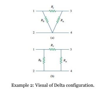
For the more daring electrical engineer, matrices can help simplify the most complex circuits that are non-linear, like a delta-delta transformer. A transformer is an electrical device that is designed on the basis of the concept of magnetic coupling. It uses magnetically coupled coils to transfer energy from one circuit to another. The transformer can be used for “stepping up” or “stepping down” AC voltages or currents. AC stands for alternating current and the voltage that was dealt with before is DC (directed current). Delta configuration represents the order of components, usually two grounded components, and one connection between them. Stating a delta-delta transformation essentially states that they are connected together.

Not all electrical engineering problems have numbers that can be solved, however that does not stop someone from making an equation for future use, once other values are known. In reality, this is actually a common practice for electrical engineers when the desired input and output is unknown.

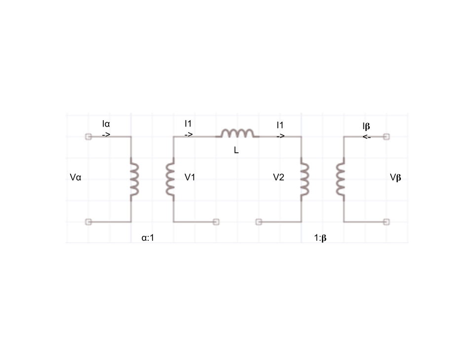
As stated before, a transformer's transfer energy comes from one circuit. Due to power conservation, the energy that may be lost or gain is still maintained within a ratio before the circuits, as shown below

The following formula was derived from the voltages on the two inductors multiple by the top inductor’s reactance

Now merge the above equations, and drive the V' and V'' from the circuit based on power conservation.

Plug and reduce, Therefore \( I_\alpha = \alpha^{-1} \left( \alpha^{-1} V_\alpha - \beta^{-1} V_\beta \right) = \alpha^{-2} V_\alpha L - (\alpha \beta )^{-1} V_\beta L . \)

because

Therefore