

Consider the initial boundary value problem:
\[
y''' + x \left( y' \right)^2 =0 , \qquad y(0) = 1 , \quad y' (0) =-2, \quad y(1) =0.
\]
We solve the given problem numerically:
ode := diff(y(x), x, x, x) + x*diff(y(x), x)^2 = 0
bics := y(0) = 1, D(y)(0) = -2, y(1) = 1
answer := dsolve({bics, ode}, numeric)
\[
\mbox{answer}:=proc(x\underscore{\ }bvp) ... end proc
\]
The output of dsolve is by default a Maple procedure of a single argument. If we call this procedure with argument x, we obtain information about the solution at that value of the independent variable:
answer(0.7)
\[
\left[ x = 0.7, \ y(x) = 0.585392388017441, \ \frac{{\text d}}{{\text d}x}\,y(x) = 0.803707863749693, \ \frac{{\text d}^2}{{\text d}x^2}\,y(x) = 3.95570431749728 \right]
\]
That is, we get a list giving us a numeric approximation to the value of the unknown and its first derivative at our choice of x. If the equation we wanted to solve was higher order (say nth order), we would have more elements in the list corresponding to all the derivatives of y up to nK1th order. The default behaviour of dsolve/numeric is to return a procedure which itself returns a list; however, we can instead have it return a list of procedures but using the optional command output = listprocedure
answer := dsolve({bics, ode}, numeric, output = listprocedure)
\[
answer:= \left[ x=proc(x) ... end proc\ ,y(x)=proc(x) ... end proc,\ \frac{{\text d}}{{\text d}x}\,y(x) = proc(x) ... end proc,\ \frac{{\text d}^2}{{\text d}x^2}\,y(x) = proc(x) ... end proc \right]
\]
Here, we get a list of three equations. The right-hand side (rhs) of each equation is a procedure that calculates what is represented on the left-hand side (lhs). For example, the rhs of the second element is a procedure that calculates y( x). We can isolate this particular procedure as follows:
y_sol := answer[2]
yy:= rhs(y_sol)
\[
yy:=proc(x) ... end proc
\]
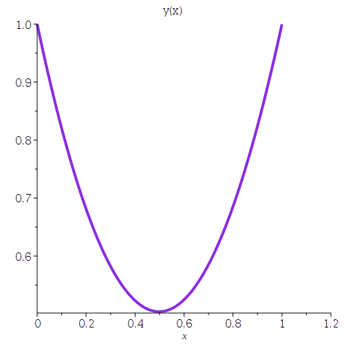
This procedure can readily be used to obtain a plot of the numeric solution of the ODE:
plot(yy(x), x = 0 .. 1.2, thickness = 4, color = "BlueViolet", title = "y(x)")
Example:
**DESCRIPTION OF PROBLEM GOES HERE**
This is a description for some Maple code. Maple is an extremely
useful tool for many different areas in engineering, applied
mathematics, computer science, biology, chemistry, and so much
more. It is quite amazing at handling matrices, but has lots of
competition with other programs such as Mathematica and Maple. Here is
a code snippet plotting two lines (y vs. x and z vs. x)
on the same graph:
(a*b)/c+13*d
ur code
another line
\[ {\frac {ab}{c}}+13\,d \]
Two n-by-n matrices A and B are called similar if there exists an invertible n-by-n matrix S such that
Theorem:
If λ is an eigenvalue of a square matrix A, then its algebraic multiplicity is at least as large as its geometric multiplicity.
▣
Let x1, x2, …
, xr be all of the
linearly independent eigenvectors associated to λ, so that
λ has geometric multiplicity r. Let
xr+1, xr+2, …
, xn complete this list to a basis for
ℜn, and let S be the n×n
matrix whose columns are all these
vectors xs, s = 1, 2, …
, n. As usual, consider the product of two
matrices AS. Because the first r columns of S are
eigenvectors, we have
\[
{\bf A\,S} = \begin{bmatrix} \vdots & \vdots&& \vdots & \vdots&&
\vdots \\ \lambda{\bf x}_1 & \lambda{\bf x}_2 & \cdots & \lambda{\bf
x}_r & ?& \cdots & ? \\ \vdots & \vdots&& \vdots & \vdots&&
\vdots \end{bmatrix} .
\]
Now multiply out S-1AS. Matrix S is
invertible because its columns are a basis for ℜn. We
get that the first r columns of S-1AS
are diagonal with &lambda's on the diagonal, but that the rest of the
columns are indeterminable. Now S-1AS has
the same characteristic polynomial as A. Indeed,
\[
\det \left( {\bf S}^{-1} {\bf AS} - \lambda\,{\bf I} \right) = \det
\left( {\bf S}^{-1} {\bf AS} - {\bf S}^{-1} \lambda\,{\bf I}{\bf S} \right) =
\det \left( {\bf S}^{-1} \left( {\bf A} - \lambda\,{\bf I} \right) {\bf S} \right) =
\det \left( {\bf S}^{-1} \right) \det \left( {\bf A} - \lambda\,{\bf
I} \right) \det \det \left( {\bf S} \right) = \det \left( {\bf A} -
\lambda\,{\bf I} \right)
\]
because the determinants of S and S-1 cancel.
So the characteristic polynomials of A and
S-1AS are
the same. But since the first few columns of
S-1AS has a factor of at least
(x - λ)r, so the algebraic multiplicity is at
least as large as the geometric.
◂
Some Text