

In the previous chapter, we show that direction fields or slope fields are very important features of differential equations because they provide a qualitative behavior of solutions. However, more precise information results from including in the plot some typical solution curves or trajectories.
A plot that shows representative sample of trajectories for a given first order differential equation is called phase portrait.
This section shows how to include sample trajectories into tangent field to obtain a phase portrait for a given differential equation.
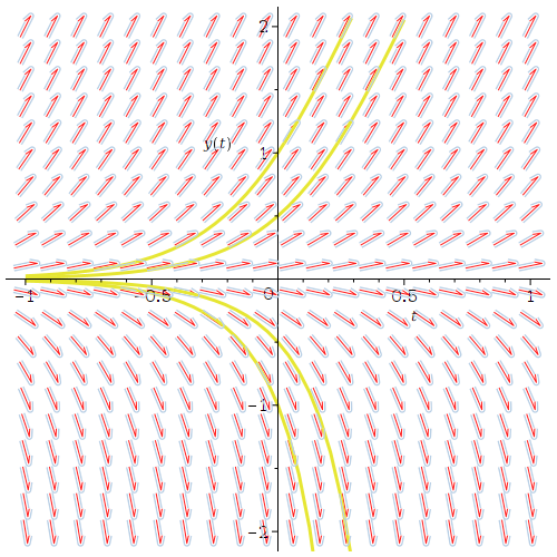
We start with a simple equample for autonomous (logistic) equation
\[
\frac{{\text d}y}{{\text d}t} = y\left( 4 - y \right) \qquad \mbox{or} \qquad \dot{y} = y\left( 4 - y \right) .
\]
The basic command in Maple to plot a direction field and some solutions is DEplots.
restart
with(DEtools):
eq := diff(y(t), t) = y(t)*(4 - y(t))
DEplot(eq, y(t), t = -1 .. 1, y = -2 .. 2, inc, [[y(0) = -1], [y(0) = 1], [y(0) = 0.5], [y(0) = -0.5]])
restart
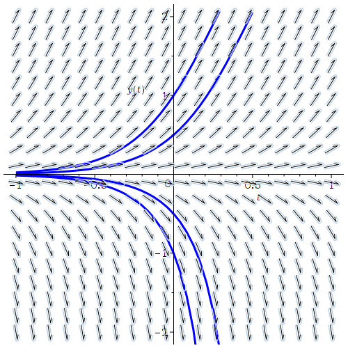
DEplot(eq, y(t), t = -1 .. 1, y = -2 .. 2, inc, [[y(0) = -1], [y(0) = 1], [y(0) = 0.5], [y(0) = -0.5]], color = black, linecolor = blue)
restart
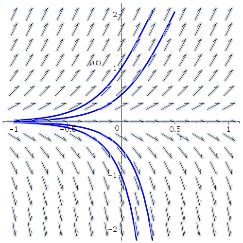
DEplot(eq, y(t), t = -1 .. 1, y = -2 .. 2, inc, [[y(0) = -1], [y(0) = 1], [y(0) = 0.5], [y(0) = -0.5]], color = black, linecolor = blue, dirgrid = [15, 15])
with(DEtools):
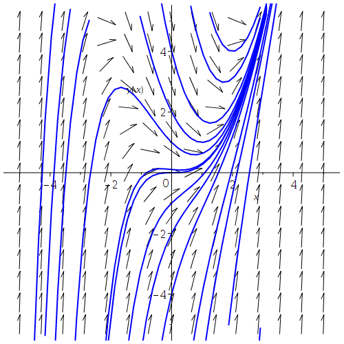
DEplot( diff(y(x),x)=x^2 - y(x), y(x), x=-5..5, y=-5..5, {[0,4],[0,2],[0,1],[0,0],[0,-1],[0,-2],[0,-4], [-4,-2],[-3,4],[-4,4],[1,4],[2,4],[3,4],[-2,-4],[1,-4],[2,-4],[3,-4]},
dirgrid=[15,15],color = black, linecolor = blue,thickness=2);
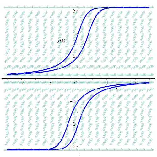
Maple has a dedicated command to plot a phase portrait:
with(DEtools):
phaseportrait(diff(y(t), t) = y(t)*sin(y(t)), y, t = -5 .. 5, [y(0) = 1, y(0) = -1, y(0) = 0, y(0) = 2, y(0) = -2], y = -Pi .. Pi, color = aquamarine, linecolor = blue)
dsolve(diff(y(x), x) = x^2 - y(x), y(x))
\[
y(x) = x^2 - 2*x + 2 + exp(-x)*{\_{ }}C1
\]
(a*b)/c+13*d
\[ {\frac {ab}{c}}+13\,d \]
Example:
**DESCRIPTION OF PROBLEM GOES HERE**
This is a description for some Maple code. Maple is an extremely
useful tool for many different areas in engineering, applied
mathematics, computer science, biology, chemistry, and so much
more. It is quite amazing at handling matrices, but has lots of
competition with other programs such as Mathematica and Maple. Here is
a code snippet plotting two lines (y vs. x and z vs. x)
on the same graph:
(a*b)/c+13*d
ur code
another line
\[ {\frac {ab}{c}}+13\,d \]
Two n-by-n matrices A and B are called similar if there exists an invertible n-by-n matrix S such that