Mathematical models utilized to describe population growth evolved, undergoing several modifications after Malthus’ model (1798).
One of the most important and well known models was proposed by the Belgium sociologist P. F. Verhulst (1838).
In this model, it is assumed that all populations are prone to suffer natural inhibitions in their growths, with a tendency to reach a steady limit value as time increases. Another important proposal was developed by Montroll (1971),
which consists of a general model, that translates the asymptotic growth of a variable taking into account the position of the inflection point of the curve.
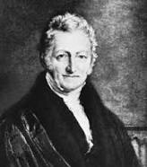
Thomas
Malthus
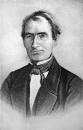
Pierre Verhulst
Growth or decay is a common occurrence in many systems ranging from biology to economics. Since mathematical language is more concise and less ambiguous than any natural language, the biological models were revised leading to the proposal of a variety of growth curves and the theoretical frameworks that lay behind them. Due to environmental trends and fluctuation, probably no biologist believes that one equation would suit all growth processes. This situation is completely different from those that we observe in physics, where usually only one law is used. For instance, modeling of the fall of a body in a vacuum requires only one of Newton's laws.
In many systems, growth patterns are ultimately subjected to some form of limitation.
In practice, we usually observe a set of measured values Yt,
at some time sequence { t }, called a time series. Modeling these observations means finding a curve P(t) that is closed to the time series. For example, to model a US population growth, we deal with an equally spaced time series, based on the census, conducted every ten years.
In this section, we discuss some simple models that are expressed solely in terms of differential equations of the first order that ignore random fluctuations in the population. Such models are referred to as deterministic and they are written as
\[
\frac{{\text d}P}{{\text d}t} = r(t,P) ,
\]
where P(t) is the size of population at time t and r is the rate of change.
A number of curve models have been developed to describe and predict such behaviors. For example, Kiviste (1988) described 75 of them in a two-volume monograph. See also the comprehensive work by Boris Zeide. There are two basic trends in population models: either autonomous differential equations or separable equations:
In many practical cases, these two approaches lead to the same population curve. Also, with different parametrizations, the same model may be written in distinct (equivalent) ways. Mathematical models to describe growth phenomena can be useful in many fields of interest including biology, ecology, medicine, or economics.
Another important example gives a tumor growth, and, in particular, cancer growth. Although cancer as well as many other tumor diseases are uncontrolled cell proliferation, developing their models may contribute to our more insightful description of changing phenomena.
Malthus and Doomsday models of population growth
With developing mathematical methods, biologists started in the late 18th century to use these techniques in population modeling in order to understand the dynamics of growing and shrinking populations of living organisms.
Thomas Malthus (1766--1834) was one of the first to note that populations grow with a geometric pattern (dP/dt = rP) while contemplating the fate of humankind. The Malthus model leads to exponential (unbounded) growth, which is clearly not viable in the long-term run:
From the formula above, a very disturbing conclusion follows: there is a finite time t = N-kk/r at which the population size becomes infinite. Therefore, the doomsday model gives more striking prediction of future catastrophe than even Malthus could come up with.
Von Foerster and his colleagues present many examples of accepted models of physical systems with singularities: pressure as a function of velocity approaching the speed of sound, current approaching breakdown voltage in gaseous conduction, index of refraction in optical absorption bands, and magnetic susceptibility at Curie temperature in ferromagnetism. It is reasonable to expect a singular behavior of a social structure subjected to extreme overpopulation. Nevertheless, the doomsday model provides a remarkably good fit of practical examples for certain time intervals.
Example:
In 1798, the English clergyman, professor, and political economist Thomas R. Malthus published anonymously a pamphlet entitled An Essay on the Principle of Population as It Affects the Future Improvement of Society, with Remarks on the Speculations of Mr. Godwin, M. Condorcet, and Other Writers.
This pamphlet was meant to counter some of the rosier utopian views of that time on the perfectibility of human society. Malthus' counter argument was that population growth would eventually produce widespread poverty or worse. His model was
\[
\frac{{\text d}P}{{\text d}t} = r\,P(t) ,
\]
where r is the per capita rate of increase –that is, how quickly the population grows per individual already in the population. If we assume no movement of individuals into or out of the population, r can be assumed to be a constant because it is just a difference of birth and death rates. Of course, this is a very simple model that has the explicit solution:
\[
P(t) = P \left( t_0 \right) e^{r \left( t - t_0 \right)} .
\]
■
Another fundamental growth mode is one subjected to limitations that affect growth rates, making growth slow down over time and asymptotically strive towards a maximum value. Growth may actually continue interminably but the rate of growth approaches zero as time tends to infinity. This is well-known in many biological systems where an organism may grow quickly in its juvenile stage but then growth slows down as it reaches maturity.
Bounded growth curves can be used to model renewable energy sources since some kind of upper limit must exist even for renewable energy.
Rather in the growth process itself,
the limiting factor lies in the form of the increasing monetary, energy, or resource costs required for continued expansion. The upper limit may be high, or virtually non-existent, but the steps in development become more and more challenging to take, thus slowing the growth process. In the biological sciences, this is often seen as proportionality between growth rate and actual size or age.
Logistic model of population growth
The best example of exponential growth is seen in bacteria. Bacteria are prokaryotes that reproduce by prokaryotic fission. This division takes about an hour for many bacterial species. If we use E. coli bacteria, we could start with just one bacterium and have enough bacteria to cover the Earth with a 30-cm layer in just 36 hours.
Usually, we never observe such exponential growth in long time run because of limitation of resources. Therefore, the Malthus model can be used only for relatively short period of time.
■
One of the most basic and milestone models of population growth was the logistic model of population growth formulated by Pierre François Verhulst in 1838. (We don't know why Verhulst called this equation logistic, but this name is universally accepted.) An outstanding exposition of its history is given by
G. Evelyn Hutchinson (1903--1991) in his book, published in 1978.
The logistic model (\( \dot{P} = r\,P \left( 1 - P/K \right) \) ) takes the shape of a sigmoid curve and describes the growth of a population. He observed that if species are not preyed upon, its population is expected to saturate. Its solution is
The relative growth rate (1/P(dP/dt) declines linearly (no maximum) with increasing population size and reaches its zero minimum at P = K, the carrying capacity, which is the maximum population size that the environment can sustain indefinitely. The population at the inflection point (where growth rate is maximum)
Example:
Using the actual data of US population given in the following table, we model it by the logistic equation with the intrinsic growth rater = 0.03 and the carrying capacityN = 10000:
First, we solve the logistic equation with the Bernoulli method by representing its solution as the product P = u v, where u is a solution of the separable equation
If one of these multiples is negative, then there does not exist a logistic curve that goes through three sequential points, as it is our case. Therefore, we need to modify the values of two points P(-10) ≈ 4.175 and P(10) ≈ 7.3 so that the logistic curve will be close to actual data.
Since that time, there has been substantial progress in developing mathematical population models.
Obviously, we cannot discuss and analyze a huge variety of population models. Instead, we present some famous models involving one ordinary differential equation. More complicated cases involving interaction of spices require a usage of system of differential equations, and this topic is covered in the second part of the tutorial.
Example:
Incorporating predation into the logistic equation may be done with the following differential equation
where P = P(t) is the population size at time t, and coefficients r, N, a, and b are some positive constants. While the logistic equation is an example of the Bernoulli equation, the above differential equation is not, but it is a separable one. However, separation of variables leads to a very complicated integral
Instead, we apply NDSolve for numerical approximations. First, we set some numerical values (r=1/20, N=1/2, 𝑎=1/10, and b=3), and then apply Mathematica.
Direction field for slope g with 1 real and 2 complex equilibria.
Direction field for slope g with 3 equilibria.
The above direction field plots allow us to determine the behavior of solutions near critical points; some of them are asymptotically stable, some only semi-stable, and others are unstable.
In each case, the variable x represents a scaled population size and the parameter 𝑎 is assumed to be positive. Both slope functions have the critical point x=0. However, the function f has an additional equilibrium pointx=1-1/ 𝑎, while the function g may have two more equilibrium points:
If 𝑎>1, then the derivative of f is positive and the critical point 1-1/𝑎 is a source (unstable). However, for 𝑎<1, the critical point is a sink (stable).
The slope function g(x) has two critical points, and the derivative at point \( x_{-}^{\ast} \) is negative for 𝑎>4; therefore, this point is asymptotically stable. The derivative of g(x) at another critical point \( x_{+}^{\ast} \) is positive for 𝑎>4. On the other hand, these two critical points disappear for 𝑎<4. So the point 𝑎=4 is a saddle-node bifurcation point.
■
Dynamics of a harvested population
Consider the dynamics of a harvested population for the logistic equation
\[
\frac{{\text d} P}{{\text d} t} = r \, P \left( 1 - \frac{P}{K} \right) - h(P) ,
\]
where r, N > 0, and where h(P) is the harvesting rate. We consider several important cases starting with a constant harvesting.
Constant harvesting
The two simplest harvesting models are constant harvesting rate and proportional harvesting rate. We start with the former.
Suppose \( h(P) = h_0 \) is a constant. Then the slope function becomes
\[
f(P) = r \, P \left( 1 - \frac{P}{K} \right) - h_0 .
\]
Setting its derivative to zero, we get \( P = \frac{1}{2}\, K . \) The function f(P) is a downward-opening parabola whose maximum value is \( f(K/2) = rK/4 - h_0 . \) Thus, if \( h_0 > rK/4 , \) the harvesting rate is too large and the population always shrinks. A saddle-node bifurcation occurs at this value of h0, and for larger harvesting rates, there are fixed points at
By rescaling the population u = P/K, time \( \tau = r\,t , \) and harvesting rate \( h = h_0 /rK , \) we arrive at the equation
\[
\dot{u} = u \left( 1 - u \right) - h .
\]
The critical harvesting rate is then \( h_c = 1/4 . \)
The proportional harvesting model is, after non-dimensionalization, of the form:
\[
\dot{u} = u \left( 1 - u \right) - h\,u .
\]
Logistic model with periodic harvesting.
T = 6.0; (* time interval length *)
ER = 8/3.; (* extraction rate *)
L = 16; (* carrying capacity *)
k = 1/3; (* exponential rate *)
b = 2.; (* low threshold *)
y1[1] = 15.; (* initial population *)
nT = 3; (* number of time cycles *)
Do[
soln1[i] =
DSolve[{y'[x] == k y[x] (1 - y[x]/L) - ER,
y[(2 i - 2) T] == y1[i]}, y[x], x] // Quiet // Flatten;
y2[i] = y[x] /. soln1[i] /. x -> T (2 i - 1);
soln2[i] =
DSolve[{y'[x] == k y[x] (1 - y[x]/L), y[(2 i - 1) T] == y2[i]},
y[x], x] // Quiet // Chop // Flatten;
y1[i + 1] = y[x] /. soln2[i] /. x -> T (2 i);
, {i, 1, nT}];
mytable =
Table[{{y[x] /. soln1[i], (2 i - 2) T <= x < (2 i - 1) T}, {y[x] /.
soln2[i], (2 i - 1) T <= x < (2 i) T}}, {i, 1, nT}];
myfun[x_] = Piecewise[Partition[Flatten[mytable], 2]];
Plot[{b, L, myfun[x]}, {x, 0, nT 2 T},
PlotRange -> {{0, nT 2 T}, {0.1, 1.1 L}}, Frame -> True,
PlotStyle -> {Dashing[0.02], Dashing[0.02], Automatic},
FrameTicks -> {T Range[0, 2 nT], Automatic, None, None},
AxesOrigin -> {0, 0}]
Rational model for harvesting
One defect of the constant harvesting rate model is that P = 0 is not a fixed point. To
remedy this, consider the following model for the harvesting rate:
\[
h(p) = \frac{a\, p^2}{p^2 + b^2} ,
\]
where 𝑎 and b are positive constants. We can rescale (N,t) to (n,τ) such that
where γ and c are positive constants. To examine the denominator of h(p), we must take P = b n. Dividing both sides of \( \dot{P} = f(P) \) by 𝑎, we obtain
\[
\frac{b}{a}\,\frac{{\text d} P}{{\text d} t} = \frac{rb}{a} \, n \left( 1- \frac{b}{N}\, n \right) - \frac{n^2}{n^2 +1} ,
\]
from which we glean τ = 𝑎t/b, γ = rb/𝑎, and c = N/b. Now we examine the scaled population model
There is an unstable fixed point at n = 0, where g'(0) = γ > 0. The other fixed points occur when the term in the brackets vanishes. We seek the intersection of the harvesting function
\( h(n) = n/(n^2 + 1) \) with a two-parameter family of straight lines, given by
\( y(n) = \gamma \left( 1- n/c \right) . \) The n-intercept is c and the y-intercept is γ. Provided c > c* is large enough, there are two bifurcations as a function of γ, which we call \( \gamma_{\pm} (c) . \)
Both bifurcations are of the saddle-node type. We determine the curves \( \gamma_{\pm} (c) \) by requiring that h(n) is tangent to y(n), which gives two equations:
Since h(n) is maximized for n = 1, where \( h(1) = \frac{1}{2} , \) there is no bifurcation occurring at value n < 1. If we plot γ(c) versus c(n) over the allowed range of n, we obtain the phase diagram. The cusp occurs at \( \left( c^{\ast} , \gamma^{\ast} \right) , \) and is determined by the requirement that the two bifurcations coincide. This supplies a third condition, namely that the second derivative is zero:
Hence, \( n = \sqrt{3} , \) which gives \( c^{\ast} = 3\sqrt{3} \quad\mbox{and} \quad \gamma^{\ast} = 3\sqrt{3} /8 . \) For c < c*, here are no bifurcations at any value of γ.
Population model with a threshold
Suppose that when the population of species falls below a certain level (called threshold, the species cannot sustain itself, but otherwise, the population follows logistic growth. To describe this situation mathematically, we introduce the differential equation
where 0 < A < B. The equilibrium solutions for this differential equation are P = 0, P = A, and P = B. To understand the dynamics of the equation, we plot the phase portrait and pahe line:
where N(t) is the size of the population at time t, r is the growth rate, and K is the equilibrium population size. Instead of the above differential equation written in a size-covariate form, it is also common to use the Gompertz model in nonautonomous form:
The Gompertz model is one of the most frequently used sigmoid models fitted to growth data and other data, perhaps only second to the logistic model.
Researchers have fitted the Gompertz model to all range of possible applications from plant growth, bird growth, fish growth, and growth of other animals, to tumour growth and bacterial growth, and the literature is enormous.
Numerous parametrisation and reparametrisations of the Gompertz model can be found in the literature, though no systematic review of these and their properties have been attempted.
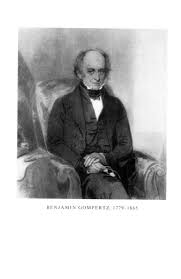
Benjamin's model is also known as the Gompertz theoretical law of mortality. He fitted it to the relationship between increasing death rate and age, what he referred to as “the average exhaustions of a man’s power to avoid death”, or the “portion of his remaining power to oppose destruction”. The insurance industry quickly started to use his method of projecting death risk. However, Gompertz only presented the probability density function.
It was W.M. Makeham who first stated this model in its well-known cumulative form, and thus it became known as the Gompertz--Makeham model.
Separation of variables in the Gompertz equation yields
The derived formulas exhitit a combination of measurable quantities--namely the tumor size N(t) and its asymptotic limiting size K--this yields a linear function of time if tumor growth. This observation plays an important role in fitting the Gompertz model to actual data. It is clear that N = K is a globally asymptotically stable fixed point, and the Gompertz model exhibits sigmoidal growth.
Next exponentiation yields the explicit formula for the Gompertz's curve:
to describe the dependence of a tree's height on its width. This equation was rediscovered several times and later was applied to model evolution of plant growths. The Korf model is motivated by the need of describing evolutionary dynamics characterized by non-zero initial values and approximately linear initial slope, and tending to a carrying capacity from below through a long-term power-law growth. We recall that various examples of population growth showing power-law behavior have been considered in the recent literature (see, for instance, Karev). It is worth pointing out that the parameters α and β are the growth and the decay rates, respectively.
The Korf differential equation is easy to solve by separating variables.
\[
\frac{{\text d}N}{N} = \alpha \left( 1 + t \right)^{-\beta -1}\,{\text d} t \qquad \Longrightarrow \qquad \ln N(t) = - \frac{\alpha}{\beta}\left( 1 + t \right)^{-\beta} + C .
\]
For small values of t the curve N(t) behaves similarly as the Gompertz curve. If α ≤ β + 1, the Korf curve has downward concavity for all t, whereas if α > β + 1, then N(t) is sigmoidal with inflection point
His model contains four common parameters: a generalised growth rate 𝑟 setting the typical time scale of the epidemic growth process, the final capacity K, which is the asymptotic total number of infections over the whole epidemics, the exponent 𝑎, which is introduced to measure the deviation from the symmetric S-shaped dynamics of the simple logistic curve, and one additional parameter 𝑎 ∈ [0,1].
Since the Richards equation is an example of a more general Bernoulli equation, we seek its solution in the form of the product R(t) = u(t) v(t), where
u(t) is a solution of the truncated linear equation
Coronavirus cases for two countries: Italy and South Africa
Days (March 1 corresponds to 1)
Actual Cases: Italy
Predicted Value of P(t)
Actual Cases: South Africa
Predicted Value of P(t)
1
1701
0
5
3858
1
9
9172
7
13
17,660
24
17
31,506
85
21
53,578
240
25
74,386
709
29
97,689
1,280
33 (April 2)
115,242
1,686
37 (April 6)
132,547
1,686
41 (April 10)
147,577
2,003
45 (April 14)
162,488
2,415
49 (April 18)
175,925
3,034
53 (April 22)
187,327
3,635
57 (April 26)
197,675
4,546
61 (April 30)
205,463
5,647
65 (May 4)
211,938
7,220
69 (May 8)
217,185
8,895
73 (May 12)
221,216
11,350
77 (May 16)
224,760
14,355
81 (May 20)
227,364
18,003
85 (May 24)
229,858
22,583
To model the data, we choose parameters: α = 0.00075, β = 23/12, and Winf = 237,000. So we get
\[
W(t) = 237,000 \left[ 1 - e^{-0.00075 \,t^{23/12}} \right] + e^{-0.00075 \,t^{23/12}} .
\]
For p < 1, this function exhibits exponential growth; and for p > 1, sigmodal growth occurs.
The von Bertalanffy model
In 1949, the Austrian biologist Karl Ludwig
von Bertalanffy (1901--1972) introduced the differential equation as a model for organism growth. He held positions at the University of Vienna (1934-48), the University of Ottawa (1950-54), the Mount Sinai Hospital (Los Angeles) (1955-58), the University of Alberta (1961-68), and the State University of New York (SUNY) (1969-72).
In 1934, he was habilitated by Reininger, Schlick and the zoologist Versluys for the first volume of his Theoretische Biologie. The monography postulated two essential aims of a theoretical biology, firstly to clean up the conceptual terminology of biology, and, secondly, to explain how the phenomena of life can spontaneously emerge from forces existing inside an organism. Here the organismic system represented the main problem as well as the still-to-be-formulated program of a theoretical biology. The second volume developed the research program of a dynamic morphology and applied the mathematical method to biological problems.
As a Rockefeller Fellow at the University of Chicago (1937-38), he worked with the Russian physicist Nicolaus Rashevsky. There he gave his first lecture about the General System Theory as a methodology that is valid for all sciences (1949). In 1939 he was appointed to an extraordinary professor at the University of Vienna. There Bertalanffy concentrated his research on a comparative physiology of growth. He was the first biologist who held lectures in zoology for students of medicine and an integrated course on botany and zoology. During this time he wrote an article about organisms as physical systems (1940), the summary of his biological reasoning: Problems of Life.
In 1949, Ludwig emigrated to Canada where he mainly worked on metabolism, growth, biophysics, and cancer cytology. In his biomedical research on cancer he developed, with his son Felix, the Bertalanffy-method of cancer cytodiagnosis. From the 1950's onwards he shifted his research from the biological sciences to the methodology of science, the General System Theory (GST), and cognitive psychology. Based on his humanistic world view, he developed a holistic epistemology (1966) which sharply criticized the machine metaphor of neobehaviorism (Robots).
In 1960 Ludwig was appointed a Professor of the Department of Zoology and Psychology at the University of Alberta in Edmonton (Canada). There Bertalanffy, the psychologist Royce and the philosopher Tenneysen established the Advanced Center for Theoretical Psychology that became a center for cognitive psychology over the next 30 years.
In that time his systematic theoretical approach focused on the modern world of technology and has thrown us humans out of nature and has isolated us from each other.
Bertalanffy emphasized in his later works the importance of the symbolic worlds of culture which we ourselves have created during evolution.
After his retirement, he became a Professor of the Faculty of Social Sciences at the State University of New York (SUNY). An international symposium celebrated his 70th birthday in 1971. In June 1972, he suffered a heart stroke and died a few days later, on June 12, shortly after midnight.
To sum up his life-work, Bertalanffy wrote 13 monographies, four anthologies, and over 200 articles, He was the chief editor of the Handbuch der Biologie--among many others. His themes encompassed theoretical biology and experimental physiology (Bertalanffy equations), theoretical psychology--particularly in the last two decades of his life, cancer research (Bertalanffy method of cancer cytodiagnosis), and philosophy and history of science.
No doubt, the person Bertalanffy was a very fascinating one, proud of his European background, a connoisseur of architectural drawings, Japanese woodcuts, and stamps, who loved to hear the music of Mozart and Beethoven and to become absorbed in the works of Goethe. Sometimes he puzzled his environment by sarcastic remarks, or his black sense of humor. His worldview was an old-fashioned one, however, never outdated that was deeply rooted in a humanistic ethos:
In the last resort, however, it is always a system of values, of ideas, of ideologies - choose whatever word you like - that is decisive. (1964)
Bertalanffy (1957) derived his equation from the assumptions, which he attributed to Pütter (1920), that the rate of anabolism is proportional to the surface area of an organism (or to its mass raised to the power of ⅔), while catabolism is proportional to the organism's mass.
Von Bertalanffy formulation (1957) of the equation is based on the biological principles of anabolism and catabolism, that is, growth and destruction. He derived his equation from the assumptions, which he attributed to Pütter (1920), that the rate of anabolism is proportional to the surface area of an organism (or to is mass raised to the power of ⅔), while catabolism is proportional to the organism's mass.
The Bertalanffy model is often used as a population model to study the factors that control and affect its growth. It is used to describe the populations of fish, animals, such as pigs, horses, cattle, sheep, etc.
It is also suitable for modelling tumors and infectious diseases because it is similar to the growth of individuals and populations:
Since the Bertalanffy equation is a Bernoully equation, we solve it by representing the solution in the form of the product of two functions: P(t) = u(t) v(t). Here u(t) is a solution of the truncated linear part:
because we need just one such solution but not the general one. Substitution of the product into the Bertalanffy equation, we obtain for v(t) the following separable differential equation:
\[
P(0) = \left[ K + C \right]^3 \qquad \Longrightarrow \qquad P^{1/3} (0) - K = C .
\]
Therefore, we finally get the solution for the von Bertalanffy model:
\[
P(t) = e^{-r\,t/K} \left[ K\,e^{r\,t/(3K)} - K + P(0)^{1/3} \right]^3 \.\to\ K \quad \mbox{as} \quad t\to \infty ,
\]
where t is time, P(0) is the population size at time t = 0, K is carrying capacity, r is the intrinsic growth rate.
This model attains its inflection value 8 K/27 at
To capture the dynamics of harvesting a population or tumour treatment we can add a harvesting term E(t) P(t). Here, E is also considered to vary with time and represents harvesting effort. Adding this term to the Bertalanffy population model results in a new harvesting IVP,
is the limit to growth parameter, β = α/η (α is a constant of integration), λ is a growth rate parameter, 1-k is a shape parameter, and the initial value is
If k > 1 and both η and λ are negative, the growth curve is sigmodal. von Bertalanffy determined empirically that k = 2/3 for a wide variety animals.
Spruce Budworm population
The spruce budworm is an insect which is a serious threat to forests.
In 1978, Ludwig, Jones, and Holling published a paper in which they
proposed an ingenious model of the interaction of the insects, the
trees, and the predatory birds. They proposed that the budworm
population P obeys a logistic model modified by a predation rate:
\begin{equation} \label{E24.6}
\frac{{\text d}P(t)}{{\text d}t} = P \left( r- \alpha P - \frac{\beta\,P}{k^2 + P^2} \right) ,
%\eqno{(4.6)}$$
\end{equation}
with some positive constants r, α, k, and β. The
parameter β represents the predation efficiency of birds and it
is proportional to the population of birds, considered a constant in
this model. The parameter k is proportional to the average leaf
surface area (about half of it), and it is a scaled measure of the
average foliage density. So trees with larger leaves attract more
budworms. The denominator, \( k^2 + P^2 , \) in the last term of the
equation models the laziness of birds that go for places where food
density is high allowing them to consume much while expending minimal
energy.
The analysis of the above equation for P(t) can be
simplified by introducing dimensionless variables \( t=a\tau \) and
P = by, where \( a= k/\beta \) and b = k. Then the equation
can be written in the following form:
where \( R=rk/\beta \) and \( A=\alpha k. \)
The above equation contains two
parameters. Its slope function has obviously one null: y = 0, but
other critical points are obtained by solving the equation
The first step in the analysis is to identify the equilibria (where the derivative of y is zero) and determine their stability.
Since the slope function is positive in a neighborhood of y = 0, this
equilibrium point is unstable. Upon multiplying both
sides of the latter equation by 1 + y², we get the cubic equation that may have
either one real root or three real roots, depending on the values of
parameters A and R. The best way to do the analysis is to examine
what can occur for each value of R as A varies.
The interpretation of the above equation is both simple and important. Its left-hand side is per capita growth
rate of the scaled variable y (with respect to a scaled time). The right-hand side is per capita death rate
due to predation, also in scaled variables. The points where these curves intersect are nonzero equilibria for
y.
The growth rate and predation loss rate of the scaled budworm density.
Two critical points
are stable and the middle is unstable.
Goel, N. S., Maitra, S. C., Montroll, E. W., On the Volterra and other nonlinear models of interacting populations. Reviews of Modern Physics, 1971, Vol. 43, pp. 231--276. https://doi.org/10.1103/RevModPhys.43.231
Gompertz B, 1825. On nature of the function expressive of the law of human mortality, and on a new mode of determining the value of life contingencies. Philosophical Transactions of the Royal Society of London, 115, 513–585.
Hutchinson, G.E., An introduction to population ecology, Yale University Press, New Haven, CT, 1978, 260p.
Janoschek A, 1957. Das reaktionskinetische Grundgesetz und seine Beziehungen zum Wachstums- und Ertragsgesetz. Statistische Vierteljahresschrift, 10, 25–37.
Kiviste, A.K., Mathematical functions of forest growth. Estonian Agricultural Academy, 1988, Tartu. 108 p + Supplement 171 p. (In Russian).
Korf, V., Contribution to the mathematical definition of forest stands growth.
(Příspěvek k matematické definici vzrůstového zákona hmot lesních porostů). Lesnická práce, 1939, Vol. 18, pp. 339--379 (In Czech).
Ludwig, D., Jones, D.D., and Holling, C.S., Journal of Animal Ecology, 1978, 47, Issue 1, 315--332.
Makeham, W.M., On the integral of Gompertz's function for expressing the values of sums depending upon the contingency of life, Journal of the Institute of Actuaries and Assurance Magazine, 1873, Vol. 17, No. 5, pp. 305--327.
Panik, M.J., Growth Curve Modeling: Theory and Applications, Wiley, 2014.
Richards, F.J., A flexible growth curve for empirical use. Journal of Experimental Botany, 1959, Vol. 10, No. 29, pp. 290--300.
Smith, D.A., Human population growth: Stability or Explosion?, Mathematics Magazine, 1977, Vol. 50, No. 4, pp. 186--197. https://www.jstor.org/stable/23686557
Thieme, H., Mathematics in Population Biology, Princeton: Princeton Univer-sity Press, 2003.
Tsoularis, A., Wallace, J., 2002. Analysis of logistic growth models. Mathematical Biosciences, 179(1), 21–55.
Verhulst, P.F., 1838. Notice sur la loi que la population suit dans son accroissement. Correspondence Mathematique et Physique, 10, 113–121.
von Bertalanffy, L, Problems of organic growth, Nature, 1949, , vol. 163, no.4135, pp. 156-158. doi:10.1038/163156a0