Preface
This is a tutorial made solely for the purpose of education and it was designed for students taking Applied Math 0330. It is primarily for students who have very little experience or have never used Mathematica before and would like to learn more of the basics for this computer algebra system. As a friendly reminder, don't forget to clear variables in use and/or the kernel.
Finally, the commands in this tutorial are all written in bold black font, while Mathematica output is in regular fonts. This means that you can copy and paste all comamnds into Mathematica, change the parameters and run them. You, as the user, are free to use the scripts to your needs for learning how to use the Mathematica program, and have the right to distribute this tutorial and refer to this tutorial as long as this tutorial is accredited appropriately.
Return to computing page for the second course APMA0340
Return to Mathematica tutorial for the second course APMA0330
Return to Mathematica tutorial for the first course APMA0340
Return to the main page for the course APMA0340
Return to the main page for the course APMA0330
Return to Part II of the course APMA0330
Direction Fields
It is also very useful to use Mathematica to graph slope fields, or direction fields. A slope field is a graph that shows the value of a differential equation at any point in a given range. These are very tiresome to do by hand, so learning how to do this with a computer algebra system is incredibly useful. In Mathematica, the only one command is needed to draw the direction field corresponding to the equation y' =1+t-y^2:
dfield = VectorPlot[{1,1+t-y^2}, {t, -2, 2}, {y, -2, 2}, Axes -> True,
VectorScale -> {Small,Automatic,None}, AxesLabel -> {"t", "dydt=1+t-y^2"}]

In this command sequence the first thing that I do is define my equation as dfield.
After this, I entered the VectorPlot command. The first equation gives me the value of {dx,dy} because the slope field graphs dy/dx or dt in this example.
Then I defined the ranges for x and t for my graphs.
By commanding the Axes-> True, I am telling Mathematica to put all of the axes on the graph.
The option VectorScale allows one to fix the size of the arrows and Normalize makes the size of the arrows be 1.
The AxesLabel command just labels the two axes on this graph.
Another thing that is very useful to do is to plot the solution to one or more initial value problems on top of the direction field.
To plot the direction field along with, for example, two solutions, we use the following commands:
sol2 = DSolve[{y'[t] == 1 - (y[t])^2 + t, y[0] == -1}, y[t], t]
pp1 = Plot[y[t] /. sol1, {t, -2, 2}]
pp2 = Plot[y[t] /. sol2, {t, -2, 2}]
Show[dfield, pp1, pp2]

In this command sequence, one first uses DSolve to solve the initial value differential equations. The third and fourth lines tells Mathematica to graph the two solutions to the initial value problem over a set range. The last command, show, tells Mathematica to show both the previously defined direction field, from the last example, and the two solutions to the differential equation. Since I just used an equal sign, =, when this command is entered I will see the solutions to the differential equations on separate graphs and then see a graph that has all three of these components on top of one another.
For plotting streamlines and their solutions, Mathematica has a dedicated command: StreamPlot. Streamlines are similar to vector lines except this command creates lines connecting the different values instead of arrows at each point.
The commands for this function are:

This is a simple command. To use StreamPlot you use almost identical syntax to VectorPlot. The only difference is that for every command in which you use "Vector," you replace this with "Stream." You can also change the aesthetics of the graph in the same manner as VectorPlot.
field = VectorPlot[{1, f[x, y]}, {x, -4, 4}, {y, -4, 4}, VectorStyle -> Arrowheads[0.025]]

NDSolve[{y'[x] == f[x, y[x]], y[0] == 0}, y, {x, -2, 2}]
graph = Plot[Evaluate[y[x] /. %], {x, -2, 2}, PlotStyle -> {Black, Thick}]


EqnB = DSolve[{y'[x]==x^2 -(y[x])^2, y[0]==-2},y[x],x]
EqnC = DSolve[{y'[x]==x^2 -(y[x])^2, y[0]==2},y[x],x]
Plot[{Evaluate[y[x]/.EqnA] , Evaluate[y[x]/.EqnB] ,Evaluate[y[x]/.EqnC]},
{x,-2,2},PlotStyle->Thickness[0.007]]

Axes->True, VectorPoints->15, VectorScale->{Tiny,Automatic,None},
StreamPoints ->8, StreamStyle->{Black,"Line"}]

Show[VectorPlot[{1, f[x, y]}, {x, -2, 2}, {y, -2, 8},
VectorStyle -> Arrowheads[0.03]],
Plot[Evaluate[Table[y[x] /. sol, {c, -10, 10, 4}]], {x, -4, 4},
PlotRange -> All]]

sol = DSolve[y'[x] == f[x, y[x]], y, x] /. C[1] -> c
Show[VectorPlot[{1, f[x, y]}, {x, -2, 2}, {y, -2, 2}, VectorStyle -> Arrowheads[0.026]],
Plot[Evaluate[Table[y[x] /. sol, {c, -10, 10, 1}]], {x, -2, 2}, PlotRange -> All]]

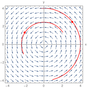
We can a point and a trajectory that goes through this point into a direction field.
Module[{vp},
vp = VectorPlot[{-y, x}, {x, -4, 4}, {y, -4, 4}, VectorScale -> {0.045, 0.9, None}, VectorPoints -> 16];
z = NDSolveValue[
Thread[{x'[t], y'[t], x[0], y[0]} == Join[{-y@t, x@t}, #]], {x@ t, y@t}, {t, -2, 1}] & /@ u;
plot = ParametricPlot[z, {t, -2, 1}, ImageSize -> 300,
Epilog -> {vp[[1]], Red, PointSize[Large], Point[u]},
PlotStyle -> Red, AspectRatio -> 1, Axes -> True,
AxesLabel -> {"x", "y"}, Frame -> True,
PlotRange -> PlotRange[vp]]], {{u, {}}, Locator,
Appearance -> None, LocatorAutoCreate -> All}, {z, {}, None}, {plot, {}, None},
Button["Print snapshot in next cell",
SelectionMove[EvaluationNotebook[], Next, Cell];
NotebookWrite[EvaluationNotebook[], ToBoxes@plot]]]