First Order Ordinary Differential Equations
This tutorial contains many Mathematica scripts. You, as the user, are free to use all codes for your needs, and have the right to distribute this tutorial and refer to this tutorial as long as this tutorial is accredited appropriately. I would like to extend my gratitude to all of the students that aided me in developing this tutorial. The coding, testing, and debugging required a concerted effort, and the following students deserve recognition for their input: Emmet and Jesse Golden-Marx (Fall 2011), Pawel Golyski (Fall 2012). Any comments and/or contributions for this tutorial are welcome; you can send your remarks to <Vladimir_Dobrushkin@brown.edu>
Return to computing page for the second course APMA0330
Return to Mathematica tutorial page for the first course
Return to Mathematica tutorial page for the second course
Return to the main page for the course APMA0330
Return to the main page for the course APMA0340
Since a differential equation includes a derivative of a function to be determined, in this context, the following notations for derivatives will be used: either the Leibniz's notation (\( {\text d}y/{\text d}x , \ {\text d}^2 y/{\text d}x^2 \) ), or Lagrange's notation (y', y''), or Newton's notation (\( \dot{y}, \ddot{y} \) ) for representing derivatives of low order with respect to time t.
First Order Differential equations
A first-order differential equation is an equation of the form
We will usually deal with differential equations where the derivative is isolated. In this case we have the differential equation in normal form:
An initial value problem for a first-order differential equation consists of the differential equation together with the specification of a value of the solution at a particular point. That is, initial value problems are of the general form:
Example: The differential equation \( y' = y \) has the solution \( y = (1/4) \left( x^2 + 2x + 1 \right) \) since \( y' = (1/2) \left( x + 1 \right) . \) This solution is defined for all real numbers. More generally, we can check that \( y' = (1/2) \left( x^2 + 2xC + C^2 \right) \) is a solution for any \( C \in \mathbb{R} . \) For the initial value problem
A general solution of a first-order differential equation is a family of solutions containing an arbitrary independent constant of integration (from some domain). A particular solution is derived from the general solution by setting the constant to particular value, often chosen to fulfill an initial condition.
A singular solution of an ordinary differential equation is a solution that cannot be obtained from the general solution \( y = \phi (x, C) \) for any choice of arbitrary constant C, including infinity, and for which the initial value problem fails to have a unique solution at some point on the solution. A singular solution in stronger sense is such function that is tangent to every solution from a family of solutions, forming the envelope of this family of solutions.
Constant functions are usually not solutions of the differential equations unless they annihilate the slope function. In this case, we call them critical points or equilibrium/stationary solutions. Therefore, if y = y* vanishes the slope function, \( f(x, y^{\ast} ) \equiv 0 , \) then y = y* is the equilibrium solution of the differential equation \( y' = f(x, y ) . \) A stationary solution may be singular or not, which we will show in the following examples.
Another class of nonlinear differential equations has a special name. Clairaut's equation (or Clairaut equation) is a differential equation of the form
Example: Consider Clairaut's equation
y=xy' + (y')^2
y[x_] = x c + c^2
samples =Table[y[x],{c,-3,3,1/4}]
Plot[Evaluate[samples],{x,-3,3},PlotRange->{-5,5}]
Out[19]= {9 - 3 x, 121/16 - (11 x)/4, 25/4 - (5 x)/2, 81/16 - (9 x)/4, 4 - 2 x,
49/16 - (7 x)/4, 9/4 - (3 x)/2, 25/16 - (5 x)/4, 1 - x,
9/16 - (3 x)/4, 1/4 - x/2, 1/16 - x/4, 0, 1/16 + x/4, 1/4 + x/2,
9/16 + (3 x)/4, 1 + x, 25/16 + (5 x)/4, 9/4 + (3 x)/2,
49/16 + (7 x)/4, 4 + 2 x, 81/16 + (9 x)/4, 25/4 + (5 x)/2, 121/16 + (11 x)/4, 9 + 3 x}
Out[20]=
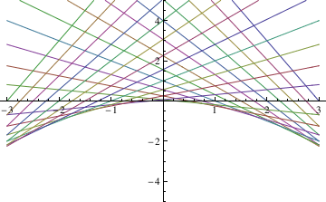
To find the singular solution (envelope), we type:
Eliminate[{x==-f'[t],y==f[t]-t*f'[t]},t]
Solving First Order ODEs
The Wolfram Language function DSolve finds symbolic solutions to differential equations. The Wolfram Language function NDSolve, on the other hand, is a general numerical differential equation solver. DSolve can handle the following types of equations:
- Ordinary Differential Equations (ODEs), in which there are two or more independent variables and one dependent variable. Finding exact symbolic solutions of ODEs is a difficult problem, but DSolve can solve many first-order ODEs and a limited number of the second-order ODEs found in standard reference books.
- Partial Differential Equations (PDEs), in which there are two or more independent variables and one dependent variable. Finding exact symbolic solutions of PDEs is a difficult problem, but DSolve can solve most first-order PDEs and a limited number of the second-order PDEs found in standard reference books.
- Differential Algebraic Equations (DAEs), in which some members of the system are differential equations and the others are purely algebraic, having no derivatives in them. As with PDEs, it is difficult to find exact solutions to DAEs, but DSolve can solve many examples of such systems that occur in applications. DSolve
Modeling with Differential Equations
Differential equations are of central importance in modeling problems in engineering, the natural sciences and the social sciences. The virtue of differential equations models rests in their ability to capture the time-evolution of processes that exhibit elements of (instantaneous) feedback. Many of the principles, or laws, underlying the behavior of the natural world are statements or reactions involving rates at which things happen. When expressed in mathematical terms, the relations are equations containing derivatives. Historically, the first equations that were studied in 18th century for modeling mechanical problems were expressed through differentials---infinitesimal quantities. This is the reason why the equations containing derivatives are referred to as differential equations but not derivative equations. The subject of differential equations is one of the most interesting and useful areas of mathematics and its applications. Technology can prove very useful when studying differential equations.
We begin our study of ordinary differential equations with first order differential equations that involve a derivative of unknown function. This tutorial contains many practical problems for which differential equations are successfully utilized. Our objective is to analyze and solve the differential equations of the normal form
A boundary value problem is one in which the function y(x) and/or some of its derivatives are specified at several distinct points.
Verification
Mathematica can be used to verify that known functions are solutions to different differential equations.
Example. To verify that the function \( y=e^{2\,x} \) is a solution of the differential equation y' - 2 y=0 type:
y[x_]=Exp[2 x]
If you enter this syntax correctly, you should get two outputs. The first output should read \( e^{2\,x} . \) You should get the second output by plugging this potential solution into the differential equation on the third line, which gives a result of zero.
As another example, consider the exponential function multiplied by a constant, \( y=c\,e^{x^2} . \) We show that this function is a solution to the differential equation \( y' -2x\, y =0 \) independently of arbitrary constant c:
Simplify[y'[x]-2 x y[x] ==0]
Out[5]= True
Some parts of the syntax of the code may be confusing, so that will be explained here. You may wonder why the variable x[k] and y[k] are used instead of x(k) and y(k). The reason is because the brackets [] resemble the denotation you see. Therefore, x[k] and y[k] in actual form would be xk and yk, respectively. The parenthesis, on the other hand, would resemble the independent variable relevant to the dependent variable in the parenthesis.
Solving First Order ODEs
Solving ODEs with the aid of standard Mathematica command: DSolvePlotting Solutions to ODEs
Direction Fields
Separable Equations
A separable equation \( y' = f(x,y) \) is such differential equation for which the slope function is a product of two functions depending on only one variable: \( f(x,y) = p(x)\,q(y) . \)Equations Reducible to the Separable Equations
We discuss some classes of differential equations that can be reduced to a separable one with an appropriate substitution.Equations with Linear Fractions
Solving equations of the form: \( \frac{{\text d}y}{{\text d}x} = f \left( \frac{ax+by+c}{Ax+By +C} \right) , \quad Ax+By +C \ne 0 . \)Exact Equations
A differential equation, written in symmetric differential form \( M(x,y)\,{\text d}x + N(x,y)\,{\text d} y =0 , \) is exact if and only if there exists a potential function ψ such that its total differential is \( {\text d}\psi (x,y) = M(x,y)\,{\text d}x + N(x,y)\,{\text d} y . \)Integrating Factors
A function μ is called an integrating factor if and only if multiplication by it reduces the differential equation \( M(x,y)\,{\text d}x + N(x,y)\,{\text d} y =0 \) to an exact equation.Linear Equations
A linear differential equation is an equation of the form \( y' + a(x)\,y = f(x) , \) where the coefficient a(x) and nonhomogeneous (also called forcing of driving) term are known continuous functions.RC circuits
Bernoulli Equations
A Bernoulli differential equation is an equation of the form \( y' + a(x)\,y = g(x)\,y^{\nu} , \) where a(x) are g(x) are given functions, and the constant ν is assumed to be any real number other than 0 or 1.Riccati Equations
A Riccati differential equation is an equation of the form \( y' + a(x)\,y = g(x)\,y^{\nu} +f(x), \quad \nu \ne 0,1 . \)Existence and Uniqueness
Peano existence theorem claims that an initial value problem \( y' = f(x,y) , \ \ y(x_0 ) = y_0 \) has a local solution if f is a continuous function. Picard--Lindelöf theorem assures us that the initial value problem has a unique solution if additionally f is also Lipschitz.Qualitative Analysis
Bifurcations
Orthogonal Trajectories
Population Models
Applications
Return to Mathematica page
Return to the main page (APMA0330)
Return to the Part 1 (Plotting)
Return to the Part 3 (Numerical Methods)
Return to the Part 4 (Second and Higher Order ODEs)
Return to the Part 5 (Series and Recurrences)
Return to the Part 6 (Laplace Transform)
Return to the Part 7 (Boundary Value Problems)