Preface
This is a tutorial made solely for the purpose of education and it was designed for students taking Applied Math 0340. It is primarily for students who have some experience using Mathematica. If you have never used Mathematica before and would like to learn more of the basics for this computer algebra system, it is strongly recommended looking at the APMA 0330 tutorial. As a friendly reminder, don't forget to clear variables in use and/or the kernel.
Finally, the commands in this tutorial are all written in bold black font, while Mathematica output is in normal font. This means that you can copy and paste all commands into Mathematica, change the parameters and run them. You, as the user, are free to use the scripts for your needs to learn the Mathematica program, and have the right to distribute this tutorial and refer to this tutorial as long as this tutorial is accredited appropriately.
Return to computing page for the second course APMA0340
Return to Mathematica tutorial for the first course APMA0330
Return to Mathematica tutorial for the second course APMA0340
Return to the main page for the course APMA0340
Return to the main page for the course APMA0330
Return to Part II of the course APMA0340
Symmetric and self-adjoint matrices
As usual, we denote by \( {\bf A}^{\ast} \) the complex conjugate and transposed matrix to the square matrix A, so \( {\bf A}^{\ast} = \overline{{\bf A}^{\mathrm T}} . \) If a matrix A has real entries, then its adjoint \( {\bf A}^{\ast} \) is just transposed \( {\bf A}^{\mathrm T} . \)
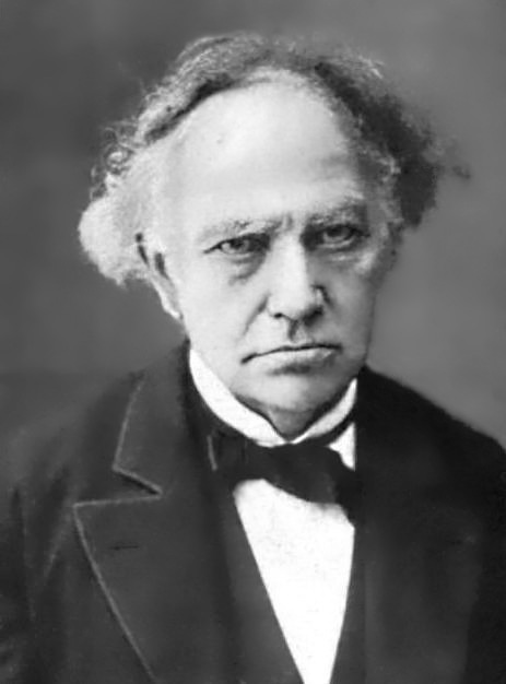
A square matrix A is called self-adjoint of Hermitian if \( {\bf A}^{\ast} = {\bf A} . \) Hermitian matrices are named after a French mathematician Charles Hermite (1822--1901), who demonstrated in 1855 that matrices of this form share a property with real symmetric matrices by always having real eigenvalues. Charles was born with a deformity in his right foot which would affect his gait for the rest of his life. He was the first to prove that e, the base of natural logarithms, is a transcendental number. His methods were later used by Ferdinand von Lindemann to prove that π is transcendental. Hermite polynomials, Hermite interpolation, Hermite normal form, Hermitian operators, and cubic Hermite splines are named in his honor. One of his students was Henri Poincaré.A square matrix Q is called unitary if \( {\bf Q} {\bf Q}^{\ast} = {\bf I} . \) If a matrix Q is unitary, then \( \det {\bf Q} = \pm 1 . \)
We formulate some properties of self-adjoint matrices.
- All eigenvalues of a self-adjoint (Hermitian) matrix are real. Eigenvectors corresponding to different eigenvalues are linearly independent.
- A self-adjoint matrix is not defective; this means that algebraic multiplicity of every eigenvalue is equal to its geometric multiplicity.
- The entries on the main diagonal (top left to bottom right) of any Hermitian matrix are necessarily real, because they have to be equal to their complex conjugate.
- Every self-adjoint matrix is a normal matrix.
- The sum or difference of any two Hermitian matrices is Hermitian. Actually, a linear combination of finite number of self-adjoint matrices is a Hermitian matrix.
- The inverse of an invertible Hermitian matrix is Hermitian as well.
- The product of two self-adjoint matrices A and B is Hermitian if and only if \( {\bf A}{\bf B} = {\bf B}{\bf A} . \) Thus, \( {\bf A}^n \) is Hermitian if A is self-adjoint and n is an integer.
- For an arbitrary complex valued vector v the product \( \left\langle {\bf v}, {\bf A}\, {\bf v} \right\rangle = {\bf v}^{\ast} {\bf A}\, {\bf v} \) is real.
- The sum of a square matrix and its conjugate transpose \( {\bf A} + {\bf A}^{\ast} \) is Hermitian.
- The determinant of a Hermitian matrix is real.
Recall that an \( n \times n \) matrix P is said to be orthogonal if \( {\bf P}^{\mathrm{T}} {\bf P} = {\bf P} {\bf P}^{\mathrm{T}} = {\bf I} , \) the identity matrix; that is, if P has inverse \( {\bf P}^{\mathrm{T}} . \) A nonsingular square complex matrix A is unitary if and only if \( {\bf A}^{\ast} = {\bf A}^{-1} . \)
Example: The matrix
sage: P*u1
sage: P*u2
sage: P*u3
Theorem: A matrix is orthogonal if and only if, as vectors, its columns are pairwise orthogonal.
Theorem: An \( n \times n \) matrix is orthogonal if and only if its columns form an orthonormal basis of \( \mathbb{R}^n . \) ■
A square matrix A is said to be orthogonally diagonalisable if there exists an orthogonal matrix P such that \( {\bf P}^{\mathrm{T}} {\bf A} {\bf P} = {\bf \Lambda} , \) where Λ is a diagonal matrix (of eigenvalues). If P in the above equation is an unitary complex matrix, then we call A unitary diagonalizable.
We can use orthogonal (or unitary) diagonalization to determine a function of a square matrix in exactly the same way as we did in diagonalization section. For instance, we can find the inverse matrix (for nonsingular matrix) \( {\bf A}^{-1} = {\bf P} {\bf \Lambda}^{-1} {\bf P}^{\mathrm T} \) and use it to solve the system of linear algebraic equations A x = b or \( {\bf P} {\bf \Lambda}^{-1} {\bf P}^{\mathrm T}\, {\bf x} = {\bf b} . \) Setting \( {\bf y} = {\bf P}^{\mathrm T} {\bf x} , \) we come across the trivial system of equations \( {\bf \Lambda}^{-1} {\bf y} = {\bf P}^{\mathrm T} {\bf b} ; \) then x = P y. ■
Theorem: An \( n \times n \) matrix A is orthogonally diagonalisable if and only if A is symmetric.
Theorem: An \( n \times n \) matrix A is unitary diagonalisable if and only if A is normal.
Example: We show that the following symmetric (but not self-adjoint) matrix is unitary diagonalizable:
sage: eigenvalues
sage: eigenvalues
sage: eigenvalues
sage: eigenvalues
Orthogonalization of a symmetric matrix: Let A be a symmetric real \( n\times n \) matrix.
Step 1: Find an ordered orthonormal basis B for \( \mathbb{R}^n ;\) you can use the standard basis for \( \mathbb{R}^n .\)
Step 2: Find all the eigenvalues \( \lambda_1 , \lambda_2 , \ldots , \lambda_s \) of A.
Step 3: Find basis for each eigenspace of A (by solving an appropriate homogeneous equation, if necessary).
Step 4: Perform the Gram--Schmidt process on the basis for each eigenspace. Normalize to get an orthonormal basis C.
Step 5: Build the transition matrix S from C, which is an orthogonal matrix and \( {\bf \Lambda} = {\bf S}^{-1} {\bf A} {\bf S} . \)
Example: Consider a symmetric matrix
sage: A =
sage: A.eigenvalues()
sage: A.fcp()
Example: The \( n \times n \) matrix with discrete Fourier transform (DFT) entries
Now we define a function of a square matrix A by \( f \left( {\bf F}_n \right) = p\left( {\bf F}_n \right) , \) which can be evaluated in \( O(n^2 \log n ) \) operations because multiplication of a vector by \( {\bf F}_n \) can be carried out in \( O(n\, \log n ) \) operations using the fast Fourier transform.
Mathematica solves linear systems
Elementary Row Operations
Row Echelon Forms
LU-factorization
PLU Factorization
Reflection
Givens rotation
Row Space and Column Space
Null Space or Kernel
Rank and Nullity
Square Matrices
Cramer's Rule
Symmetric and self-adjoint matrices
Cholesky decomposition
Projection Operators
Gram-Schmidt
QR-decomposition
Least Square Approximation
SVD Factorization
Numerical Methods
Markov chains
Inequalities
Miscellaneous
Return to Mathematica page
Return to the main page (APMA0330)
Return to the Part 1 Matrix Algebra
Return to the Part 2 Linear Systems of Equations
Return to the Part 3 Linear Systems of Ordinary Differential Equations
Return to the Part 4 Non-linear Systems of Ordinary Differential Equations
Return to the Part 5 Numerical Methods
Return to the Part 6 Fourier Series
Return to the Part 7 Partial Differential Equations