2.2.9. Sigular Value Decomposition

SVD factorization ¶

One of the most fruitful ideas in the theory of matrices is that of matrix decomposition or canonical form. The theoretical utility of matrix decompositions has long been appreciated. Previously, we have discused LU-decomposition and QR-factorization for rectangular m-by-n matrices. For a square \( n \times n \) matrix, we know even more canonical forms:

• An eigenvalue decomposition (abbreviated EVD) of a symmetrical (self-adjoint) matrix
  \[ {\bf A} = {\bf P}\,{\bf \Lambda}\,{\bf P}^{\mathrm T} \qquad \mbox{or} \qquad {\bf A} = {\bf P}\,{\bf \Lambda}\,{\bf P}^{\ast} . \]
  where P is an n-by-n orthogonal (unitary) matrix of eigenvalues of A, and Λ is the diagonal matrix whose diagonal entries are eigenvalues corresponding to the column vectors of S.
• A Hessenberg decomposition of a square matrix with real entries, due to the German electrical engineer Karl Hessenberg (1904--1959),
  \[ {\bf A} = {\bf P}\,{\bf H}\,{\bf P}^{\mathrm T} , \]
  in which P is an orthogonal matrix and H is in upper Hessenberg form: \( {\bf H} = \begin{bmatrix} x&x & \cdots &x&x&x \\ x&x& \cdots &x&x&x \\ 0&x& \cdots&x&x&x \\ \vdots&\vdots & \ddots &\vdots& \vdots& \vdots \\ 0&0& \cdots &x&x&x \\ 0&0& \cdots &0&x&x \end{bmatrix} . \)
• Schur's decomposition for an n-by-n matrix A with real entries and real eigenvalues: \( {\bf A} = {\bf P}\,{\bf S}\,{\bf P}^{\mathrm T} , \) where P is an orthogonal matrix such that \( {\bf P}^{\mathrm T} {\bf A} \, {\bf P} = \begin{bmatrix} \lambda_1 & x & x& \cdots & x \\ 0&\lambda_2 & x & \cdots & x \\ 0&0&\lambda_3& \cdots & x \\ \vdots&\vdots& \vdots & \ddots & \vdots \\ 0&0&0& \cdots & \lambda_n \end{bmatrix} , \) in which \( \lambda_1 , \lambda_2 , \ldots , \lambda_n \) are the eigenvalues of A repeated according to multiplicity.
• Cholesky decomposition of a positive definite matrix: \( {\bf A} = {\bf L}\,{\bf L}^{\ast} , \) where L is a lower triangular matrix.

Of many useful decompositions, the singular value decomposition---that is, the factorization of a m-by-n matrix A into the product \( {\bf U}\, {\bf \Sigma} \,{\bf V}^{\ast} \) of a unitary (or orthogonal) \( m \times m \) matrix U, a \( m \times n \) 'diagonal' matrix \( {\bf \Sigma} \) and another unitary \( n \times n \) matrix \( {\bf V}^{\ast} \) ---has assumed a special role. There are several reasons. In the first place, the fact that the decomposition is achieved by unitary matrices makes it an ideal vehicle for discussing the geometry of n-space. Second, it is stable; small pertubations in A corresponds to small pertubabtions in \( {\bf \Sigma} .\) Third, the diagonality of \( {\bf \Sigma} \) makes it easy to operate and solve equations.

It is an intriguing observation that most of the classical matrix decompositions predated the widespread use of matrices. In 1873, the Italian mathematician Eugenio Beltrami (1835--1899) published a first paper on SVD, which was followed by the work of Camille Jordan in 1874, whom we can consider as a codiscover. Later James Joseph Sylvester (1814--1897), Edhard Schmidt (1876--1959), and Hermann Weyl (1885--1955) were responsible for establishing the existence of the singular value decomposition (SVD) and developing its theory. The term ``singular value'' seems to have come from the literature on integral equations. The British-born American mathematician Harry Bateman (1882--1946) used it in a research paper published in 1908.

• \( {\bf A}^{\ast} {\bf A} \) and \( {\bf A} \, {\bf A}^{\ast} \) are both symmetric positive semidefinite matrices of dimensions \( n \times n \) and \( m \times m ,\) respectively.
• The equality \( {\bf A} = {\bf U}\,{\bf \Sigma}\, {\bf V}^{\ast} = {\bf U}\,{\bf \Sigma}\, {\bf V}^{-1} \) is called the singular value decomposition (or SVD) of A, where V is unitary (or orthogonal in real-valued case) \( n \times n \) matrix, U is unitary/orthogonal \( m \times m \) matrix, and \( {\bf \Sigma} = {\bf U}^{\ast} {\bf A}\, {\bf V} \) is diagonal \( m \times n \) matrix, with \( {\bf \Sigma} = \mbox{diag}( \sigma_1 , \sigma_2 , \ldots , \sigma_p ), \) where \( p = \min (m,n) \) and the nonnegative numbers \( \sigma_1 \ge \sigma_2 \ge \cdots \ge\sigma_p \ge 0 \) are singular values of A.
• If r is rank of A, then A has exactly r positive singular values \( \sigma_1 \ge \sigma_2 \ge \cdots \ge\sigma_r > 0 \) with \( \sigma_{r+1} = \sigma_{r+2} = \cdots = \sigma_p =0 . \)
• Any real \( m \times n \) matrix A can be expressed as a finite sum of rank 1 matrices in normalized form, that is, \( {\bf A} = \sigma_1 {\bf R}_1 + \sigma_2 {\bf R}_2 + \cdots + \sigma_r {\bf R}_r , \) where \( {\bf R}_i = {\bf u}_i {\bf v}_i^{\ast} = {\bf u}_i \otimes {\bf v}_i , \) \( {\bf u}_i \) is the i-th column of U and a unit vector of \( {\bf A}\,{\bf A}^{\ast} , \) and \( {\bf v}_i \) is the i-th column of V and a unit eigenvector of \( {\bf A}^{\ast} {\bf A} . \)
• The pseudoinverse \( {\bf A}^{\dagger} \) of a matrix with SVD \( {\bf A} = {\bf U}\,{\bf \Sigma}\, {\bf V}^{\ast} \) is the matrix \( {\bf A}^{\dagger} = {\bf V} {\bf \Sigma}^{\dagger} {\bf U}^{\ast} \) with
  \[ {\bf \Sigma}^{\dagger} = \mbox{diag} \left( \frac{1}{\sigma_1} , \cdots , \frac{1}{\sigma_r} , 0, \cdots , 0\right) \in \mathbb{R}^{m\times n} . \]

Theorem: If A is an \( m \times n \) matrix with real entries, then

• A and A^TA have the same null space (kernel).
• A and A^TA have the same row space.
• A^T and A^TA have the same column space.
• A and A^TA have the same rank.

Theorem: If A is an \( m \times n \) real matrix, then

• A^TA is orthogonally diagonalizable: \( {\bf V}^{\mathrm T} \left( {\bf A}^{\mathrm T} {\bf A} \right) {\bf V} = \mbox{diag} \left( \sigma_1^2 , \ldots , \sigma_n^2 \right) . \)
• The eigenvalues \( \{ \sigma_1^2 , \ldots , \sigma_n^2 \} \) of A^TA are nonnegative.
• The column vectors of U are the eigenvectors of the symmetric matrix AA^T. ■

Example. Consider the matrix

Definition: If A is an \( m \times n \) matrix, and if \( \lambda_1 , \lambda_2 , \ldots , \lambda_n \) are the eigenvalues of A^TA, then the numbers

are called the singular values of A. In other words, a nonnegative real number σ is a singular value for m-by-n matrix A if and only if there exist unit-length vectors \( {\bf u} \in \mathbb{R}^m \quad\mbox{and} \quad {\bf v} \in \mathbb{R}^n \) such that \( {\bf A}{\bf v} = \sigma {\bf u} . \) The vectors u and v are called left singular and right singular vectors for σ, respectively. ■

Theorem: Let A be a m-by-n matrix with complex or real entries. Then its largest singular value equals to the Euclidean 2-norm: \( \max \{ \sigma_i \} = \| {\bf A} \|_2 = \max_{\| {\bf x} \| =1} \| {\bf A} {\bf x} \| , \) and square root of the sum of squares of the singular values equals the Frobenius norm: \( \sum_i \sigma_i^2 = \| {\bf A} \|_F^2 = \sum_{i,j} |a_{i,j} |^2 = \mbox{trace} \left( {\bf A}^{\ast} {\bf A} \right) . \) ■

There are known two forms of the singular value decompositions---the brief (or reduced) version and the expanded form:

Theorem: (Singular Value Decomposition in expanded form) If A is an \( m \times n \) matrix of rank r, then A can be factored as

• \( {\bf V} = \left[ {\bf v}_1 \ {\bf v}_2 \ \cdots \ {\bf v}_n \right] \) orthogonally diagonalizes \( {\bf A}^{\mathrm T} {\bf A} = {\bf V} \mbox{diag} (\sigma_i^2 ) \,{\bf V}^{\mathrm T} .\) Column vectors in V are usually called right singular vectors of A.
• The nonzero diagonal entries of Σ are \( \sigma_1 = \sqrt{\lambda_1} , \ \sigma_2 = \sqrt{\lambda_2} , \ldots , \sigma_r = \sqrt{\lambda_r} , \) where \( \lambda_1 , \lambda_2 , \ldots , \lambda_r \) are the nonzero eigenvalues of A^TA corresponding to the column vectors of V.
• The column vectors of V are ordered so that \( \sigma_1 \ge \sigma_2 \ge \cdots \ge \sigma_r >0. \)
• \( {\bf u}_i = \frac{{\bf A} {\bf v}_i}{\| {\bf A} {\bf v}_i \|} = \frac{1}{\sigma_i} \, {\bf A}\,{\bf v}_i \quad (i=1,2,\ldots , r) . \)
• \( {\bf U} = \left[ {\bf u}_1 , {\bf u}_2 , \ldots , {\bf u}_r \right] \) is an orthogonal basis for the column space of A. Column vectors in U are usually called left singular vectors of A.
• \( \left[ {\bf u}_1 , {\bf u}_2 , \ldots , {\bf u}_r , {\bf u}_{r+1} , \ldots , {\bf u}_m \right] \) is an extension of \( \left[ {\bf u}_1 , {\bf u}_2 , \ldots , {\bf u}_r \right] \) to an orthogonal basis for \( {\mathbb R}^m . \) ■

When rank r of \( m \times n \) matrix A is less than \( \min \{ m, n \} , \) the most entries of 'diagonal' \( m \times n \) matrix Σ are zeroes except singular values \( \sigma_1 , \ldots , \sigma_r . \) Therefore, when this matrix is multiplied from left by U and from right by V^T, their entries \( {\bf u}_{r+1} , \ldots , {\bf u}_m \) and \( {\bf v}_{r+1} , \ldots , {\bf v}_n \) do not contribute to the final matrix. So we can drop them and represent A in the reduced form, as the following theorem states.

Let r be the rank of m-by-n matrix A. Then \( \sigma_{r+1} = \sigma_{r+2} = \cdots = \sigma_n . \) Partition \( {\bf U} = \left[ {\bf U}_1 \ {\bf U}_2 \right] \) and \( {\bf V} = \left[ {\bf V}_1 \ {\bf V}_2 \right] , \) where \( {\bf U}_1 = \left[ {\bf u}_1 \ , \ldots , \ {\bf u}_r \right] \) and \( {\bf V}_1 = \left[ {\bf v}_1 \ , \ldots , \ {\bf v}_r \right] \) have r columns. Then with \( {\bf \Sigma}_r = \mbox{diag}(\sigma_1 , \ldots , \sigma_r ) : \)

Theorem: (Singular Value Decomposition in brief/reduced form) If A is an \( m \times n \) matrix of rank r, then A can be expressed in the form \( {\bf A}_{m\times n} = {\bf U}_{m\times r} {\bf \Sigma}_r {\bf V}^{\mathrm T}_{r\times n} , \) where Σ_r has size r-by-r and

The matrices U and V are not uniquely determined by A, but the diagonal entries of Σ are necessarily the singular values of A. The set \( \{ {\bf u}_1 , \ldots , {\bf u}_r \} \) is an orthonormal basis for the column space of A. The set \( \{ {\bf u}_{r+1} , \ldots , {\bf u}_m \} \) is an orthonormal basis for the kernel (null space) of A^T. The set \( \{ {\bf v}_1 , \ldots , {\bf v}_r \} \) is an orthonormal basis for the row space of A. The set \( \{ {\bf v}_{r+1} , \ldots , {\bf v}_n \} \) is an orthonormal basis for the kernel of A.

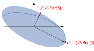
Example. If \( {\bf A} = \left[ \begin{array}{ccc} 1\ & 2& \ 6 \\ 2\ & -3 \ & -2 \end{array} \right] , \) then the linear transformation \( {\bf x} \,\mapsto \,{\bf A}{\bf x} \) maps the unit sphere \( \left\{ {\bf x} : \, \| {\bf x} \| =1 \right\} \) in \( {\bf \mathbb R}^3 \) onto an ellipse in \( {\bf \mathbb R}^2 , \) shown in Figure:

The singular values of A are the square roots of the eigenvalues of \( {\bf B}_1 = {\bf A}^{\mathrm T} {\bf A} : \)

Now we construct the orthogonal matrices

Example. Consider the full rank matrix

Example. Consider a 3-by-2 matrix \( {\bf A}^{\mathrm T} = \begin{bmatrix} 4& -1&1 \\ -4 & 1& -1 \end{bmatrix} . \) First, we compute two symmetric singular matrices:

Example. However,