Preface

---

This is a tutorial made solely for the purpose of education and it was designed for students taking Applied Math 0340. It is primarily for students who have some experience using Mathematica. If you have never used Mathematica before and would like to learn more of the basics for this computer algebra system, it is strongly recommended looking at the APMA 0330 tutorial. As a friendly reminder, don'r forget to clear variables in use and/or the kernel.

Finally, the commands in this tutorial are all written in bold black font, while Mathematica output is in regular fonts. This means that you can copy and paste all comamnds into Mathematica, change the parameters and run them. You, as the user, are free to use the scripts to your needs for learning how to use the Mathematica program, and have the right to distribute this tutorial and refer to this tutorial as long as this tutorial is accredited appropriately.

Contents [hide]

• Introduction
• 1. Part I: Matrix Algebra
     1. How to define Vectors
     2. How to define Matrices
     3. Basic Operations with Matrices
     4. Linear Systems of Equations
     5. Determinants and Inverse Matrices
     6. Special Matrices
     7. Eigenvalues and Eigenvectors
     8. Generalized Eigenvectors
     9. Diagonalization Procedure
     10. Sylvester Formula
     11. The Residue Method
     12. Spectral Decomposition Method
     13. Positive Matrices
     14. Roots
     15. Miscellaneous
  2. Part II: Linear Systems of Equations
     1. Matrices and Vectors
     2. Mathematica solves linear systems
     3. Elementary Row Operations
     4. Row Echelon Forms
     5. LU-factorization
     6. PLU Factorization
     7. Reflection
     8. Givens rotation
     9. Row Space and Column Space
     10. Null Space or Kernel
     11. Rank and Nullity
     12. Square Matrices
     13. Cramer's Rule
     14. Symmetric and self-adjoint matrices
     15. Cholesky decomposition
     16. Projection Operators
     17. Gram-Schmidt
     18. QR-decomposition
     19. Least Square Approximation
     20. SVD Factorization
     21. Numerical Methods
     22. Markov chains
     23. Inequalities
     24. Applications
  3. Part III: Linear Systems of Ordinary Differential Equations
     1. Solving ODEs
     2. Direction Fields
     3. Separable Equations
     4. Equations Reducible to the Separable Equations
     5. Exact Equations
     6. Integrating Factors
     7. Linear and Bernoulli Equations
     8. Riccati Equations
     9. Existence and Uniqueness
     10. Qualitative Analysis
     11. Applications
     12. References
  4. Part IV: Non-linear Systems of Ordinary Differential Equations
     1. Numerical Solution using DSolve and NDSolve
     2. Euler's Methods
     3. Polynomial Approximations
     4. Runge-Kutta Methods
     5. Multistep Methods
     6. Numerov Method
     7. Applications
     8. References
  5. Part V: Numerical Methods
     1. Fundamental Set of Solutions
     2. General Solutions of Homogeneous Equations
     3. Reduction of Order
     4. Variation of Parameters/Lagrange
     5. Method of Undetermined Coefficients
     6. Operator Method
     7. Applications
     8. References
  6. Part VI: Fourier Series
     1. Definition
     2. Periodic Functions
     3. Complex Fourier Series
     4. Examples
     5. Cesaro summation
     6. Gibbs Phenomenon
     7. Even and odd functions
     8. Chebyshev expansions
     9. Legendre expansion
     10. Bessel expansion
     11. Hermie expansion
     12. Motivated Examples from Music
  7. Part VII: Partial Differential Equations
     1. Heat Conduction Problems
     2. Other Heat transfer equations
     3. Wave equations
     4. Transverse Vibrations of Beams
     5. Laplace Equation
     6. Laplace Equation in Polar Coordinates
     7. Applications
     8. References

Return to computing page for the first course APMA0330
Return to computing page for the second course APMA0340
Return to Mathematica tutorial for the first course APMA0330
Return to Mathematica tutorial for the second course APMA0340
Return to the main page for the course APMA0340
Return to the main page for the course APMA0330

 

2.2.4. Reflection

---

 

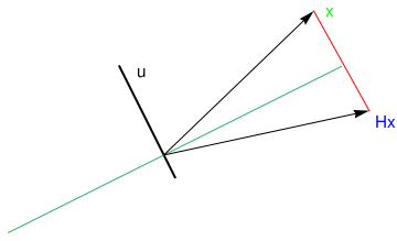
Reflection

Suppose that we are given a line spanned over the vector a in \( \mathbb{R}^n , \) and we need to find a matrix H of reflection about the line through the origin in the plane. This matrix H should fix every vector on line, and should send any vector not on the line to its mirror image about the line. The subspace \( {\bf a}^{\perp} \) is called the hyperplane in \( \mathbb{R}^n , \) orthogonal to a. The \( n \times n \) orthogonal matrix

\[ {\bf H}_{\bf a} = {\bf I}_n - \frac{2}{{\bf a}^{\mathrm T} {\bf a}} \, {\bf a} \, {\bf a}^{\mathrm T} = {\bf I}_n - \frac{2}{\| {\bf a} \|^2} \, {\bf a} \, {\bf a}^{\mathrm T} \]

is called the Householder matrix or the Householder reflection about a, named in honor of the American mathematician Alston Householder (1904--1993). The complexity of the Householder algorithm is \( 2mn^2 - (2/3)\, n^3 \) flops (arithmetic operations). The Householder matrix \( {\bf H}_{\bf a} \) is symmetric, orthogonal, diagonalizable, and all its eigenvalues are 1's except one which is -1. Moreover, it is idempotent: \( {\bf H}_{\bf a}^2 = {\bf I} . \) When \( {\bf H}_{\bf a} \) is applied to a vector x, it reflects x through hyperplane \( \left\{ {\bf z} \, : \, {\bf a}^{\mathrm T} {\bf z} =0 \right\} . \)

Householder, Alston, S. Principles of Numerical Analysis, New York, McGraw Hill, 1953.

P := {-3, -1}; Q := {3, 2};
lineseg = Graphics[{RGBColor[0.2, 0.7, 0.4], Line[{P, Q}]}]
u = Graphics[{Black, Thick, Line[{{0, 0}, {-1, 2}}]}]
ar1 := Graphics[Arrow[{{-0.2, 0.4}, {5/2, 3}}]]
ar2 := Graphics[Arrow[{{-0.2, 0.4}, {3.5, 1.2}}]]
line2 = Graphics[{RGBColor[1, 0, 0], Line[{{5/2, 3}, {3.5, 1.2}}]}]
textu = Graphics[Text[Style["u", FontSize -> 14, Black], {-0.6, 1.9}]]
textx = Graphics[Text[Style["x", FontSize -> 14, Red], {2.8, 3.0}]]
textHx = Graphics[Text[Style["Hx", FontSize -> 14, Blue], {3.8, 1.0}]]
Show[u, lineseg, ar1, ar2, line2, textu, textx, textHx]

Example. We present some simple reflections on the plane and in 3D in the following tables.

Operator	Illustration	Standard Matrix
Reflection about the x-axis T(x,y) = (x,-y)		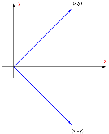\( \begin{bmatrix} 1&0 \\ 0&-1 \end{bmatrix} \)
Reflection about the y-axis T(x,y)=(-x,y)		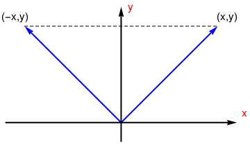\( \begin{bmatrix} -1&0 \\ 0&1 \end{bmatrix} \)
Reflection about the line y=x T(x,y)=(y,x)		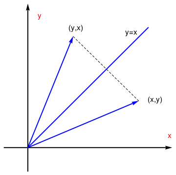\( \begin{bmatrix} 0&1 \\ 1&0 \end{bmatrix} \)

Operator	Illustration	Standard Matrix
Reflection about the xy-plane T(x,y,z) = (x,y,-z)		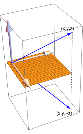\( \begin{bmatrix} 1&0&0 \\ 0&1&0 \\ 0&0&-1 \end{bmatrix} \)
Reflection about the xz-plane T(x,y,z)=(x,-y,z)		\( \begin{bmatrix} 1&0&0 \\ 0&-1&0 \\ 0&0&1 \end{bmatrix} \)
Reflection about the yz-plane T(x,y,z)=(-x,y,z)		\( \begin{bmatrix} -1&0&0 \\ 0&1&0 \\ 0&0&1 \end{bmatrix} \)

Example. Consider the vector \( {\bf u} = \left[ 1, -2 , 2 \right]^{\mathrm T} . \) Then the Householder reflection with respect to vector u is

Theorem: If u and v are distinct vectors in \( \mathbb{R}^n \) with the same norm, then the Householder reflection about the hyperplane \( \left( {\bf u} - {\bf v} \right)^{\perp} \) maps u into v and conversely. ■

We check this theorem for two-dimensional vectors \( {\bf u} = \left[ u_1 , u_2 \right]^{\mathrm T} \) and \( {\bf v} = \left[ v_1 , v_2 \right]^{\mathrm T} \) of the same norm. So given \( \| {\bf v} \| = \| {\bf u} \| , \) we calculate

Example. We find a Householder reflection that maps the vector \( {\bf u} = \left[ 1, -2 , 2 \right]^{\mathrm T} \) into a vector v that has zeroes as its second and third components. Since this vecor has to be of the same norm, we get \( {\bf v} = \left[ 3, 0 , 0 \right]^{\mathrm T} . \) Since \( {\bf a} = {\bf u} - {\bf v} = \left[ -2, -2 , 2 \right]^{\mathrm T} , \) the Householder reflection \( {\bf H}_{{\bf a}} = \frac{1}{3} \begin{bmatrix} 1&-2&2 \\ -2&1&2 \\ 2&2&1 \end{bmatrix} \) maps the vector \( {\bf u} = \left[ 1, -2 , 2 \right]^{\mathrm T} \) into a vector v. Matrix \( {\bf H}_{{\bf a}} \) is idempotent (\( {\bf H}_{{\bf a}}^2 = {\bf I} \) ) because its eigenvalues are -1, 1, 1. ■

sage: nsp.is_finite()
False

We use the Householder reflection to obtain an alternative version of LU-decomposition. Consider the following m-by-n matrix:

Algorithm (Row-oriented vertion of Householder transformations):

Step 1: Compute \( \sigma_a \) and β

Step 2: Compute the factor row \( \left( \alpha , {\bf w}^{\mathrm T} \right) : \)

Step 3: Apply Gaussian elimination using the pivot row and column from step 2:

This formulation of Householder transformations can be regarded as a special kind of Gauss elimination, where the pivot row is computed from a linear combination of the rows of the matrix, rather than being taken directly from it. The numerical stability of the process can be seen from the fact that \( |z_i | \le 1 \) and \( |w_j | \le \beta \le 2 \) for every entry in z and w.

The Householder algorithm is the most widely used algorithm for QR factorization (for instance, qr in MATLAB) because it is less sensitive to rounding error than Gram--Schmidt algorithm.