Adomian Decomposition Method

---

This tutorial surves as an introduction to the computer algebra system Maple, created by MapleSoft ©. It is made solely for the purpose of education. This tutorial assumes that you have a working knowledge of basic Maple functionality. It is recommended to switch to Maple Classic so all codes will have the same appearance, regardless of the version used. To achieve this, follow the following steps:

• when Maple is open, select "tools" at the top, and then "Options;"
• click on the "Display" tab, and in the "Input display" select "Maple Notation;"
• click on the "Interface" tab and in the "Default format for new worksheets" select "Worksheet;"
• go to the bottom of the "Options" menu and click on the "Apply Globally."
• Now close Maple and open it again

Usually, the same algorithm can be implemented in many different ways to accomplish the same task. As a result, this tutorial may introduce several different commands (or sets of commands) to do the same thing. It is always good to be aware of these alternate pathways; however, you are welcome to pick up any approach whatever you like the best .

Finally, the commands in this tutorial are all written in red text (as Maple input), while Maple output is in blue, which means that the output is in 2D output style. You can copy and paste all commands into Maple, change the parameters and run them. You, as the user, are free to use the mw files and scripts to your needs, and have the rights to distribute this tutorial and refer to this tutorial as long as this tutorial is accredited appropriately. The tutorial accompanies the textbook Applied Differential Equations. The Primary Course by Vladimir Dobrushkin, CRC Press, 2015; http://www.crcpress.com/product/isbn/9781439851043.

Adomian Decomposition Method

The Adomian decomposition method (ADM) is a semi-analytical method for solving ordinary and partial nonlinear differential equations. The method was developed from the 1970s to the 1990s by an American mathematician and aerospace engineer of Armenian descent George Adomian (1922-1996), chair of the Center for Applied Mathematics at the University of Georgia. The crucial aspect of the method is employment of the "Adomian polynomials" to represent the nonlinear portion of the equation as a convergent series with respect to these polynomials, without actual linearization of the system. These polynomials mathematically generalize Maclaurin series about an arbitrary external parameter, which gives the solution method more flexibility than direct Taylor series expansion.

Let me introduce some scientists (in alphabetic order) who contributed and greatly improved Adomian Decomposition Method to make it available to mathematical and engineering community.

Dr. George Adomian (1922--1996) was an American mathematician, theoretical physicist, and electrical engineer of Armenian descent. He received his Ph.D. degree from UCLA. He first proposed and considerably developed the Adomian Decomposition Method (ADM) for solving nonlinear differential equations, ordinary, and partial. He was a professor of mathematics at the University of Georgia, the founder and chief scientist of General Analytics Corporation, a winner of the 1989 Richard Bellman Prize for outstanding contributions to nonlinear stochastic analysis, and a National Academy of Sciences Scholar 1988. He is the author of eight books on and over three hundred journal papers.

Dr. Adomian was the Radar Officer (naval rank of Lieutenant, the equivalent of a Captain in the Army by direct commission) aboard the USS Antietam (CV-36), and served in the Pacific Theater of Operations during the Second World War. He also attended the secret radar school at MIT which trained the first radar officers for the U.S. Navy.

Dr. Yves Cherruault (1937--2010) was a French mathematician. He received his Ph.D. degree from the University of Paris. He was a professor of mathematics at the University Pierre et Marie Curie, Paris, and the Director of MÉDIMAT (Laboratory of Mathematics Applied to Biomedicine). Professor Cherruault is one of the founders of the field of Biomathematics and an author of seven books and over two hundred journal papers. Dr. Cherruault developed some of the convergence theorems of the ADM.

Dr. Jun-Sheng Duan is a Chinese applied mathematician and computer scientists born in Inner Mongolia, China, in 1965. He received his Ph.D. degree from Shandong University, China. He has extensive contributions to solutions of differential equations in mathematical physics and engineering using ADM and the Modified Decomposition Method (MDM) in collaboration with Drs. Rach and Wazwaz. He has been a professor of mathematics at the Inner Mongolia Polytechnic University, the Tianjin University of Commerce, and currently at the School of Sciences, Shanghai Institute of Technology, China. He is the author of more than eighty journal papers.

Dr. Duan is an outstanding player of wei qi (the Chinese “game of go”), and ping-pong (table tennis). He enjoys photography and traveling.

Dr. Randolph Rach is a retired Army veteran and formerly a Senior Engineer at Microwave Laboratories Inc. His experience includes research and development in microwave electronics and traveling-wave tube technology, and his research interests span nonlinear system analysis, nonlinear ordinary and partial differential equations, nonlinear integral equations and nonlinear boundary value problems. He published more than one hundred and thirty papers in applied mathematics, and he is an early contributor to the ADM. Dr. Rach’s fundamental theorems established the basis for the early development of ADM. He was also the first to propose the MDM. His past and current research continue to advance the state of the art of ADM/MDM.

Dr. Sergio E. Serrano was born in Santander (Colombia) in 1953. He is a professor of environmental engineering, hydrologic science, applied mathematics, and philosophy at Temple University in Philadelphia. He received his Ph.D. degree at the University of Waterloo (Canada). He has more than one hundred research publications in international science, engineering, and mathematical journals. He is also the author of eight books in environmental engineering, statistics, philosophy, and psychology. Dr. Serrano has been awarded four times with nationally-competitive research grants by the National Science Foundation, Washington, DC. Using adaptations and modifications of the ADM, he has developed hundreds of practical engineering models of flood wave propagation, contaminant transport, and groundwater flow in irregular geometries.

Dr. Serrano has a passion for hiking. In 1973, he explored on foot the rain forest of the Darien Sierra from Acandi (Colombia) to Yaviza (Panama). He plays the recorder (Renaissance flute). He enjoys alchemy, archaeology, home wine making, herbal medicine, and cooking. He believes that the joy of meaningful living, and meaningful relationships, can be found in the simplicity of everyday life. He lives in Philadelphia with his wife of thirty years and his daughter.

Dr. Abdul-Majid Wazwaz is a Professor of Mathematics at Saint Xavier University in Chicago. He received his Ph.D. from the University if Illinois at Chicago. He was the author and co-author of more than four hundred and fifty papers in applied mathematics and mathematical physics. He is the author of five books on the subjects of discrete mathematics, integral equations and partial differential equations. He has contributed extensively to theoretical advances in solitary waves theory, the ADM, and other computational methods. He is a member of the editorial board of the journals Nonlinear Dynamics (Springer) and Physica Scripta (IOP). For these three years in a row, 2014, 2015, and 2016, Thomas Reuters granted him three different badges for being a “Highly Cited Researcher.”

We show how the method works in the series of examples. Since the Adomian method has its roots in quantum mechnaics and operator methods, we need to reconsider our old friend---the derivative operator. It is convenient to set a special symbol for the derivative operator, which is naturally denoted by \( \texttt{D} = {\text d} / {\text d} x . \) Its inverse is studied in calculus, and we denote it as

where the initial point of integration, s = 0 was chosen for simplicity (any point from the domain of y(s) will work) and \( y(0) = y_0 . \) Of course, the derivative operator is defined on the space of smooth functions and its inverse acts in the space of integrable (for instance, in Riemann sense) functions. It should be noted that such defined operator \( \texttt{D}^{-1} \) is only right inverse to the derivative operator: \( \texttt{D}\,\texttt{D}^{-1} = \texttt{I} , \) which is the identity operator. Note that application of \( \texttt{D}^{-1} \) to the derivative yields

Example. Let us take a constant function \( y(x) \equiv 1 , \) then

where C is a constant of integration. The derivative of y(x) is identically zero, so So we see that \( \texttt{D} \) and \( \texttt{D}^{-1} \) do not commute. ■

Example. We start with a simple initial value problem for linear equation:

where a is a constant. Introducing the derivative operator \( \texttt{D} = {\text d} / {\text d} x , \) we rewrite the linear differential equation as where Assuming that the solution is the inifinite sum we substitute this series into either the differential equation or the formula Comparing like terms, we get the recurrence relation Each of these recurrences is actually a linear difference-differential equation, which is easy to solve: and so on. Adding all these terms, we get the solution The first constant term can be dropped and we have \( y(x) = y_0 e^{-ax} . \) ■

Example. Our next example is also related to the linear differential equation, but now we consider variable coefficient nonhomogeneous equation:

Expanding the unknown solution y as \( y(x) = \sum_{k\ge 0} y_k , \) and substituting into the differential equation, we obtain Clearly y₀ in the above equation is a solution of the initial value problem: This is a calculus problem and Maple easily solves it: Therefore, \( y_0 (x) = \frac{5}{2} + \frac{x^2}{2} . \) Any other subsequent term is derived from the recurrence: We solve this recurrence using Maple: This gives first five approximations: and \( y_5 = \frac{1}{1440} \left( 35 - 174 x^2 + 345 x^4 -340 x^6 + 165 x^8 - 30 x^{10} - x^{12} \right) . \) Adding these terms, we get 5-term approximation to the actual solution \( y(x) = \frac{1}{2} + \frac{5}{2}\,e^{1-x^2} : \) We plot the actual solution in blue and approximation in orange: From the above graph, we see that the ADM solution \( \phi_5 (x) \) is almost undistinguishable from the exact within the interval [1, 1.5]. However, for \( x \ge 1.6 , \) the ADM solution begins to diverge from the exact one. This is typical: the convergence rate is a function of the window of observation. If number of terms in ADM approximation is taken more, the approximate solution improves at high values x. From here we conclude that as x increases, the number of ADM terms needed to obtain an accurate solution increases. ■

Now we turn our attention to initial value problems for nonlinear equations such as

where we have chosen the initial point to be the origin for simplicity. Here a(t), b(t), and f(t) are known and bounded functions in variable t, and N[y] is a nonlinear (analytic) operator acting on dependent variable (function) y(t). As before, we define the derivative operator \( \texttt{D} = {\text d}/ {\text d}t \) with respect to independent variable t and rewrite the given initial value problem in operator form: The main idea of the Adomian decomposition method is to represent the nonlinear term as the sum of so called Adomian polynomials: where A_n are the Adomian polynomials specifically generated for each nonlinear operator according to the formula: In particular, For the approximations of the solution \( y = u_0 + u_1 + u_2 + \cdots \) and the nonlinear operator \( N[y] = A_0 + A_1 + A_2 + \cdots \) correspond ordinary generating functions where λ is a parameter. The decomposition method consists in identifying the u_n's by means of the formulae

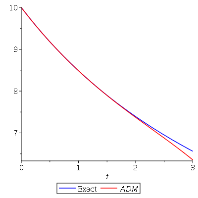
Example. We apply Adomian decomposition method to find approximate solution to the initial value problem for logistic equation:

This problem has a unique solution as Maple confirms We expand the nonlinear term N[P] = P² into the series: where first five polynomials are not hard to determine manually: Substituting expansion \( P = u_0 + u_1 + u_2 + \cdots \) into the given logistic equation, we get For the first term, we have the initial value problem Solving the initial value problem for the above linear equation we get the first term: For next terms, we have which is a linear differential equation with respect to u_n. Solving these equations recursively, we obtain restart: y[0]:=t->y0: #Initial condition
N:=y->y^2: #Nonlinear term
A[0]:=N(y0):
0.02*int(y[0](t),t)-0.02*int(A[0],t):
y[1]:=unapply(%,t):
Nt:=5:
for n from 1 to Nt do
diff( N(sum(y[m](t)*lambda^m,m=0..n)),lambda$n)/n!:
A[n]:=subs(lambda=0,%);
0.02*int(y[n](t),t)-0.02*int(A[n],t):
y[n+1]:=unapply(%,t);
end do:
sum(y[i](t),i=0..Nt):
phi:=unapply(%,t): #ADM approximate solution
Y:=t->10*exp(t/50)/(10*exp(t/50)-9): #Exact solution
Then we plot the exact solution in blue and ADM approximation in red: y0:=10: T:=3:
g1:=plot(Y(t),t=0..T,color=blue,legend="Exact "):
g2:=plot(phi(t),t=0..T,color=red,legend=ADM):
plots[display](g1,g2);
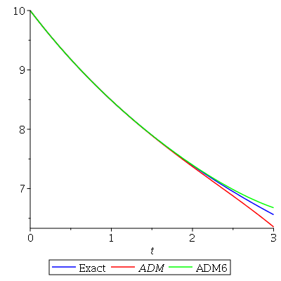
To see how ADM appfroximation works, we add one more polynomial to obtain ADM six term approximation. g3 := plot(phi(t)+55506619*t^6/(125*10^9), t = 0 .. T, color = green, legend = "ADM6")
plots[display](g1, g2, g3)
As we see, the ADM approximation with six terms (green) is more accurate to the actual solution (in blue) than the ADM approximation with five terms (in red).

Example. Consider the initial value problem for the integro-differential equation

Using ADM method, we seek approximate solution in the form where \( u_0 =50 \) and nonlinear operator N[y] is expanded into Adomian polynomials: Since we have Now we are ready to construct 6-term ADM approximation Using Mathematica we obtain