Second and Higher Order Ordinary Differential Equations
This web site provides an introduction to the computer algebra system Maple, created by MapleSoft ©. This tutorial is made solely for the purpose of education, and intended for students taking APMA 0330 course at Brown University.
The commands in this tutorial are all written in red text (as Maple input), while Maple output is in blue, which means that the output is in 2D output style. You can copy and paste all commands into Maple, change the parameters and run them. You, as the user, are free to use the mw files and scripts to your needs, and have the rights to distribute this tutorial and refer to this tutorial as long as this tutorial is accredited appropriately. The tutorial accompanies the textbook Applied Differential Equations. The Primary Course by Vladimir Dobrushkin, CRC Press, 2015; http://www.crcpress.com/product/isbn/9781439851043. Any comments and/or contributions for this tutorial are welcome; you can send your remarks to <Vladimir_Dobrushkin@brown.edu>
Return to computing page for the first course APMA0330
Return to computing page for the second course APMA0340
Return to Maple tutorial for the first course APMA0330
Return to Maple tutorial for the second course APMA0340
Return to the main page for the first course APMA0330
Return to the main page for the second course APMA0340
1.4.1. Solving Higher Order Linear ODEs
Example 1.4.1: Consider a second order differential equation
Then we apply the phaseportrait function to obtain:
DE1 := diff(y(t),t) = z(t);
DE2 := diff(z(t),t) = -y(t)*cos(y(t));
phaseportrait([DE1,DE2],[y,z],t=-5..5,[[y(0)=1,z(0)=0],[y(0)=0,z(0)=2],[y(0)=0,z(0)=-2]],y=-Pi..Pi,z=-3..3,color=aquamarine,linecolor=blue);
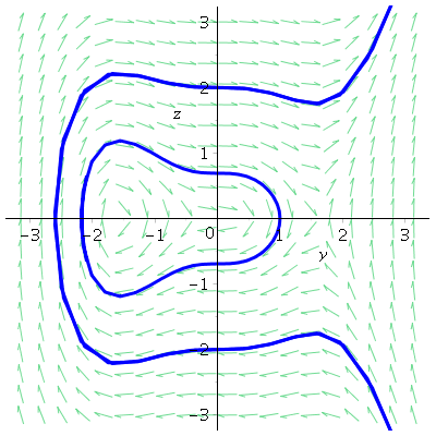
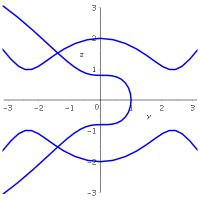
There are a few things worth noting here. First, the solution curves are traced both forwards and backwards in time. Without actually plotting a point where the initial conditions are located, you will not be able to identify the initial point. Second, note that the function plots a direction field for autonomous equations, but does not do that for the 2-D case if the equation is not autonomous. Changing the equation to \( y' = z, \quad z' = -y cos t \) and applying the phaseportrait function to that
DE1 := diff(y(t),t) = z(t);
DE2 := diff(z(t),t) = -y(t)*cos(t);
phaseportrait([DE1,DE2],[y,z],t=-5..5,[[y(0)=1,z(0)=0],[y(0)=0,z(0)=2],[y(0)=0,z(0)=-2]],y=-Pi..Pi,z=-3..3,color=aquamarine,linecolor=blue);
produces the plot
Example 1.4.2:
II. Plotting
1.3. Separable Equations
A differential equation y' = f(x,y) is said to be separable if the slope function is the product of two functions depending on only one variable: f(x,y) = p(x) q(y). Then rewriting the derivative y' in differential form y' = dy / dx , we separate variables:
dy / q(y) = p(x) dx
each part can be integrated. In other words, a separable differential equation is a differential equation in which the two variables can be placed on opposite sides of the equals sign such that the dx and x terms are on one side and the dy and the y terms are on the other. The dx and dy terms need to be multiplied by the x and y terms, respectively.
There are two methods that can be used to solve the solution to a separable differential equation. We show these methods on the follwoing example.
Example 1.3.1. Consider separable differential equation: y'= xy/(1+x*x). We show two methods that can be used to solve the given separable differential equation. A first one is to ask Matlab to find the solution.
Example 1.3.2. Consider separable differential equation: y' +ycos(x) =0
Example 1.3.3. Consider separable differential equation: x(y+1)(y-3) dx +(1+5y)(x+2) dy =0. We solve this equation by separating variables and then integrating:
1.4. Equations Reducible to the Separable Equations
Example 1.4.1.
Solutions to the equation xy'=x^2 y^3 -y
Example 1.4.3. Consider the initial value problem
y' = 1/(x-y+2), y(0) =1 . We find its solution (in implicit form) and prot it using the following Mathematica's commands: Example 1.4.4.
Another example.
Example 1.4.5.
Consider the differential equation
dy/dx = ( (2x-2y-2) / {x-1})^2 , where x != 1
We exclude the singular point x=1 where the
integral curves have an infinite slope. The right-hand side
function (= slope function) is a composition of two functions:
( (2x-2y-2) / (x-1) )^2 = F(z(x,y)) , where F(z) = z^2 and z = (2x-2y-2) / (x-1) .
The function F(z(x,y)) is not homogeneous, but it can be converted to a homogeneous one by shifting
x=X+\alpha and y=Y+\beta ,
where
\alpha = 1, \beta = 0
so x=X+1, \ y=Y. We next substitute $x=X+1$ and $y=Y$ into the given
equation and simplify. The result is
dY/dX = dy / d(x-1) = dy /dx = {2(x-1)
-2y/{x-1} )^2 = ( (2X -2Y) / X )^2
Setting $Y=vX$ gives us
X dv /dX +v = 4 (1-v)^2 or dv (4(1-v)^2 -v) = dX / X .
Plotting the direction field, it can be seen that $v = a /2 \approx 1.64039$ is unstable equilibrium solution, and $v=
\frac{b}{2} \approx 0.609612$ is a stable equilibrium solution. These
critical points are not singular solutions because integral curves do
not touch them, which means that an initial value problem for the
differential equation $X\,v' = (2v-a)(2v-b)$ has a unique solution.
Now we return to the original variables. Since $X=x-1, \ Y=y$, and
$v=Y/X$, the original differential equation has the general solution
in implicit form:
C|x-1|^{\sqrt{17}} = \left| \frac{8y -(9 + \sqrt{17})(x-1)}{8y -(9 -\sqrt{17})(x-1)} \right| , x ! = 1.
It can be solved with respect to $y$, and then plotted using the following Mathematica commands:
The given differential equation has two equilibrium solutions that correspond to $v=a/2$ and $v=b/2$:
y = (x-1) a/2 = (x-1) (9+\sqrt{17) )/8 and
y = (x-1) b/2 = (x-1) (9-\sqrt(17)) /8.