MuPAD Tutorial. First Course: Exact Equations

Recall the total differential of a function ψ(x,y) of two variables, denoted by dψ, is given by the expression

\[ {\text d}\psi (x,y) = \frac{\partial \psi}{\partial x} \,{\text d}x + \frac{\partial \psi}{\partial y} \, {\text d}y . \]

Let M(x,y) and N(x,y) be two smooth functions having continuous partial derivatives in some domain \( \Omega \subset \mathbb{R}^2 \) without holes. A differential equation, written in differentials

\[ M(x,y)\,{\text d}x + N(x,y)\, {\text d}y =0 \]

is called exact if and only if

\[ \frac{\partial M(x,y)}{\partial y} = \frac{\partial N(x,y)}{\partial x} \]

or there exists a smooth function \( \psi (x,y) ,\) called the potential function, such that its total differential

\[ {\text d}\psi = M(x,y)\,{\text d}x + N(x,y)\, {\text d}y =0 \qquad \mbox{or} \qquad \frac{\partial \psi}{\partial x} = M(x,y), \quad \frac{\partial \psi}{\partial y} = N(x,y). \]

A potential function is not unique to which arbitrary constant can be added. Once it is known, the general solution is obtained immediately:

\[ \psi (x,y) = C , \qquad \mbox{a constant}. \]

There are two approaches to find a potential function corresponding to an exact equation. The first one is based on integration of

\[ M(x,y) = \frac{\partial \psi}{\partial x} , \qquad N(x,y) = \frac{\partial \psi}{\partial y} \qquad \mbox{or using shortcut}\qquad M = \psi_x , \quad N= \psi_y \]

because the total differential of ψ is \( {\text d} \psi = \psi_x {\text d}x + \psi_y {\text d} y \) for all \( x \in \Omega . \) The second method utilizes line integration, which is preferred for solving initial value problems. Indeed, suppose we are given an initial value problem for an exact equation:

\[ M(x,y)\,{\text d}x + N(x,y)\, {\text d}y =0 , \qquad y(x_0) = y_0 . \]

Let L be arbitrary curve starting at \( (x_0 ,y_0 ) \) and ending at arbitrary point \( (x,y) . \) This curve or line should be without self-intersections and belong to the domain Ω where functions M(x,y) and N(x,y) possess continuous derivatives. Then the potential function can be obtained as

\[ \psi (x,y) = \int_L M(x,y)\,{\text d}x + N(x,y)\, {\text d}y . \]

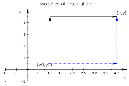
In practice, we choose L as a semi-linear line going parallel to axes from initial point \( (x_0 ,y_0 ) \) and finishing at arbitrary point \( (x,y) \in \mathbb{R}^2 . \) In particular, we can integrate first along vertical axis and then horizontally, or we can integrate horizontally and then vertically.

window:=plot::Arrow2d([-1,-1],[-1,-1],LineColor=RGB::Blue)
line1:=plot::Arrow2d([1,.5],[4,.5],LineColor=RGB::Blue,LineStyle=Dashed,Title="(x0,y0)",TitlePosition=[.75,.25])
line2:=plot::Arrow2d([4,.5],[4,4.5],LineColor=RGB::Blue,LineStyle=Dashed,Title="(x,y)",TitlePosition=[4.2,4.7])
line3:=plot::Arrow2d([1,.5],[1,4.5],LineColor=RGB::Black)
line4:=plot::Arrow2d([1,4.5],[4,4.5],LineColor=RGB::Black)
plot(window,line1,line2,line3,line4,Header="Two Lines of Integration")

If we integrate along black line (vertically where dx = 0 and then horizontally where dy = 0), we get

\[ \psi (x,y) = \int_{y_0}^y N(x_0 ,y)\, {\text d}y + \int_{x_0}^x M(x ,y)\,{\text d}x . \]

Now if we integrate along blue dashed line (horizontally where dy = 0 and then vertically where dx = 0), we get

\[ \psi (x,y) = \int_{x_0}^x M(x ,y_0 )\,{\text d}x + \int_{y_0}^y N(x ,y)\, {\text d}y . \]

Example: The equation \( y \,\text{d}x + x \,\text{d}y =0 \) is exact because \( M_y =1 = N_x \) for \( M= y \quad\mbox{and} \quad N= x . \) Suppose that the initial condition \( y(2)=3 \) is given.

We type in MuPad:

reset()
M:=y

N:=x

initcondx:=2

initcondy:=3

3
Check to see if this equation is exact

is(diff(M,y)=diff(N,x))

TRUE
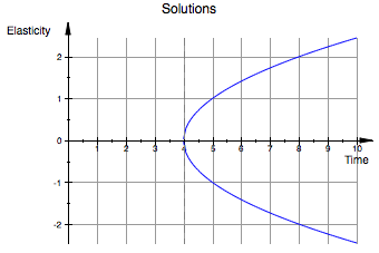
Check that integrating along either the black line (Psi1) or the blue line (Psi2) will give the same solution

Psi1:=simplify(int(M,x=initcondx..x)+int(2,y=initcondy..y))

x y - 6

Psi2:=simplify(int(3,x=initcondx..x)+int(N,y=initcondy..y))

x y - 6

Example: Consider the differential equation

\[ \left( x+ 2y \right) {\text d}x + \left( 2x-3y \right) {\text d}y =0. \]

First, we check whether the given equation is exact.

M:=x+2*y

x + 2 y

N:=2*x-3*y

2 x - 3 y
Check to see that the equation is exact.

is(diff(M,y)=diff(N,x))

TRUE
Solve for Ψ.

F:=int(M,x)

\( \displaystyle \frac{x \left( x + 4\,y \right)}{2} \)

Derfy:=diff(F,y)-N

3 y

fofy:=int(Derfy,y)

\( \displaystyle \frac{3\, y^2}{2} \)

psi1:=F+fofy

\( \displaystyle \frac{x \left( x + 4\,y \right)}{2} + \frac{3\, y^2}{2} \)

Example: Consider the initial value problem for the exact differential equation:

\[ \frac{5}{x}\, y' + \left( \ln x -1 \right) y + 4x=0, \qquad y(1 ) = 1 . \]

We find its solution by typing:

IVP4:= ode({5*y(x)/x+4*x+(ln(x)-1)*y'(x)=0, y(1) = 1}, y(x))
solve(IVP4)

To plot more than one function on the same graph, you can separate them by commas as different parameters in the same plot function.

plot(function1, function2, x=start..end, y=start..end)

When defining a function to plot (separate from inside the plot function), sometimes it is nice to include a parameter for the line color - 'LineColor = RGB::Red' - which literally stands for 'choose between red green and blue for your line'.

curve1 := plot::Function2d(function3,t=0..10, LineColor = RGB::Red)

Notice that there is an extra identifier in front of the plot function this time '::Function2d'. This is just to indicate to MuPad that we want it to be a 2 dimensional graph in cases of a 3 dimensional object. In the case where you are plotting objects of multiple variables, this can be very useful. To get a 3 dimensional graph, all you have to do is change the '2' above to a '3'.

Labels are used as parameters inside the plot function. The syntax is as follows: 'Header = ['This Is My Title']' and 'AxesTitles = ['Xaxis Title', 'YAxis Title']'. Here is an example with all the aspects at once:

curve1 := (sqrt(x -4),LineColor = RGB::Blue)
curve2 := (-sqrt(x -4))
plot(curve1,curve2, x=0..10, y=-5..5, Header = 'Solutions', AxesTitles = ['Time','Elasticity'],GridVisible = TRUE)