Electric Circuits

A circuit is an unbroken loop of conductive material that allows electrons to flow through continuously without beginning or end. If a circuit is “broken,” that means its conductive elements no longer form a complete path, and continuous electron flow cannot occur in it. The location of a break in a circuit is irrelevant to its inability to sustain continuous electron flow. Any break, anywhere in a circuit prevents electron flow throughout the circuit.

When charge flows through the wires of an electric circuit, current is said to exist in the wires. Electric current is a quantifiable notion which is defined as the rate at which charge flows past a point on the circuit. It can be determined by measuring the quantity of charge that flows past a cross-sectional area of a wire on the circuit. As a rate quantity, current (I) is expressed by the following equation:

where \( q \) is the quantity of charge flowing by a point in a time period of t. The standard metric unit for the quantity current is the ampere, often abbreviated as Amps or A. A current of 1 ampere is equivalent to 1 Coulomb of charge flowing past a point in 1 second. The conventional symbol for current is I, which originates from the French phrase intensité de courant, meaning current intensity. Current intensity is often referred to simply as current. The I symbol was used by André-Marie Ampère (1775--1836), after whom the unit of electric current is named, in formulating the eponymous Ampère's force law, which he discovered in 1820. Since the quantity of charge passing a point on a circuit is related to the number of mobile charge carriers (electrons) which flow past that point, the current can also be related to the number of electrons and the time. To make this connection between the current and the number of electrons, one must know the quantity of charge on a single electron.

As charge flows through a circuit, it encounters resistance or a hindrance to its flow. Like current, resistance is a quantifiable term. The quantity of resistance offered by a section of wire depends upon three variables - the material the wire is made out of, the length of the wire, and the cross-sectional area of the wire. One physical property of a material is its resistivity - a measure of that material's tendency to resist charge flow through it. Resistivity values for various conducting materials are typically listed in textbooks and reference books. Knowing the resistivity value ( \( \rho \) ) of the material the wire is composed of and its length (L) and cross-sectional area (A), its resistance (R) can be determine using the equation below.

Resistors are used to keep wire conductors from receiving too much current. Consisting of a material with low permittivity, the resistor reduces electron flow and thus lowers the current, saving items such as LED’s from melting due to high current flow.

The standard metric unit of resistance is the ohm (abbreviated by the Greek letter \( \Omega \) ). The main difficulty with the use of the above equation pertains to the units of expression of the various quantities. The resistivity ( \( \rho \) ) is typically expressed in ohm•m. Thus, the length should be expressed in units of m and the cross-sectional area in \( m^2 \). Many wires are round and have a circular cross-section. As such, the cross-sectional area in the above equation can be calculated from knowledge of the wire's radius or diameter using the formula for the area of a circle.

The amount of current that flows in a circuit is dependent upon two variables. Current is inversely proportional to the overall resistance (R) of the circuit and directly proportional to the electric potential difference impressed across the circuit. The electric potential difference (ΔV) impressed across a circuit is simply the voltage supplied by the energy source (batteries, outlets, etc.). For homes in the United States, this value is close to 110-120 Volts. The mathematical relationship between current (I), voltage and resistance is expressed by the following equation (which s sometimes referred to as the Ohm's law equation):

Electrical circuits are all about energy. Energy is put into a circuit by the battery or the commercial electricity supplier. The elements of the circuit (lights, heaters, motors, refrigerators, and even wires) convert this electric potential energy into other forms of energy such as light energy, sound energy, thermal energy and mechanical energy. Power refers to the rate at which energy is supplied or converted by the appliance or circuit. It is the rate at which energy is lost or gained at any given location within the circuit. As such, the generic equation for power is The energy loss (or gain) is simply the product of the electric potential difference between two points and the quantity of charge which moves between those two points in a time period of t. As such, the energy loss (or gain) is simply ΔV • Q. When this expression is substituted into the above equation, the power equation becomes Since the Q/t ratio found in the above equation is equal to the current (I), the above equation can also be written as By combining the Ohm's law equation with the above equation, two other power equations can be generated. They are

The standard metric unit of power is the Watt.

It is quite common that a circuit consist of more than one resistor. While each resistor has its own individual resistance value, the overall resistance of the circuit is different than the resistance of the individual resistors which make up the circuit. A quantity known as the equivalent resistance indicates the total resistance of the circuit. Conceptually, the equivalent resistance is the resistance that a single resistor would have in order to produce the same overall effect on the resistance as the combination of resistors which are present. So if a circuit has three resistors with an equivalent resistance of 25 ohm, then a single 25-ohm resistor could replace the three individual resistors and have the equivalent effect upon the circuit. The value of the equivalent resistance ( \( R_{eq} \) ) takes into consideration the individual resistance values of the resistors and the way in which those resistors are connected.

There are two basic ways in which resistors can be connected in an electrical circuit. They can be connected in series or in parallel. Resistors which are connected in series are connected in consecutive fashion such that all the charge that passes through the first resistor will also pass through the other resistors. In series connection, all of the charge flowing through the circuit passes through all the individual resistors. As such, the equivalent resistance of series-connected resistors is the sum of the individual resistance values of those resistors.

Resistors which are connected in parallel are connected in side-by-side fashion such that the charge approaching the resistors will split up into two or more different paths. Parallel-connected resistors are characterized as having branching locations where charge branches off into the different pathways. The charge which passes through one resistor will not pass through the other resistors. The equivalent resistance of parallel-connected resistors is less than the resistance values of all the individual resistors in the circuit. While it may not be entirely intuitive, the equation for the equivalent resistance of parallel-connected resistors is given by an equation with several reciprocal terms.

 

Inductors are used to reduce the change in current. Usually made up of wire conductors wrapped in coils, inductors create a “back emf” (in Henrys) inverse to the change in the magnetic field flux caused by changing current. Proportional to the change in current, this emf (electromotive force) increases for large changes in the current smoothing out the current over time. Because inductors pass low frequencies much more easily than high frequencies, they are often used as filters on sub-woofers in speaker systems. The reason to use an inductor there is that it doesn't "consume" or "waste" the high frequency energy, it just blocks it from passing, so that energy can then pass through the capacitor, to the tweeter, instead.

When an inductor and resistor are placed in sequence in a circuit powered by a battery of emf \( \varepsilon_0 \) (see fig below) the voltage given by a combination of Ohm’s and Kirchhoff’s law is:

where the emf of inductance is \( L\,\frac{{\text d}I}{{\text d} t} .\) This can be rearrange as the separable first order differential equation \( \frac{{\text d}I}{{\text d} t} = \varepsilon_0 /L -I\,R/L .\) Separating \( I(t) \) and \( t \) and integrating, we get: where \( C \) is an arbitrary constant. If we have zero current \( I(0) =0 \) at time \( t=0, \) then solving for \( C, \) we get \( C= - \varepsilon_0 /R . \) Raising both sides of the equation \( \ln \left( \frac{\varepsilon_0 - I\,R}{\varepsilon_0} \right) = -t\,R/L \) to \( e, \) and solving for \( I(t), \) we get the general solution to the differential equation: The following mupad code can be used to solve and graph the solution given a starting voltage of 30 V, an inductance of 25 mH, and a resistance of 3 \( \Omega . \) For the first second, the current increases, but not instantaneously because of the inductor. Then by two seconds the current reaches its steady state, V/R, because the inductance part of the equation, \( e^{Rt/L} , \) drops to zero as the current reaches its maximum for the circuit and stops changing.

An LC circuit is a closed loop with just two elements: a capacitor and an inductor. It has a resonance property like mechanical systems such as a pendulum or a mass on a spring: there is a special frequency that it likes to oscillate at, and therefore responds strongly to. LC circuits can be used to tune in to a specific frequency, for example in the station selector of a radio or television.

In an LC circuit, electric charge oscillates back and forth just like the position of a mass on a spring oscillates. To demonstrate the analogy, we list several corresponding equations for a mechanical spring and an LC circuit.

Mechanical spring	LC circuit
position x	charge q
velocity \( v= \dot{x} = \frac{{\text d}x}{{\text d}t} \)	current \( I = \dot{q} = \frac{{\text d}q}{{\text d}t} \)
kinetic energy \( \frac{1}{2}\, mv^2 \)	Inductor energy \( \frac{1}{2}\, L\, I^2 \)
potential energy \( \frac{1}{2}\, k x^2 \)	Capacitor energy \( \frac{1}{2} \left( \frac{1}{C} \right) q^2 \)
equation of motion \( m\,\dot{v} + k\,x =0 \)	Kirchhoff's law \( L\,\frac{{\text d}I}{{\text d}t} + \frac{q}{C} =0 \)
frequency \( \frac{1}{2\pi} \, \sqrt{\frac{k}{m}} \)	frequency \( \frac{1}{2\pi} \, \frac{1}{\sqrt{LC}} \)

The parameters that determine the motion of a spring are the mass m, spring constant k, the position x, and the velocity v which is the rate of change of x. The parameters that determine the behavior of an LC circuit are L, C, q and I which is the rate of change of q. Thus there is a one-to-one correspondence since the equations of motion are identical given the substitutions:

 

The characteristic frequency of an LC circuit is the frequency at which large amplitudes are built up when a driving force is applied at that frequency. A child on a swing will be sensitive to a pushing force which comes regularly with the natural frequency of the swing. A force that comes at a different frequency will not build up a large amplitude as it will often be pushing against the child's motion. The magic frequency is called the resonant frequency.

First, we will create an RC-circuit with the resistor and capacitor in series. We need to create variables (wire1, res1, res2, etc.) that hold a plot of a line segment that will be part of our circuit, then we need to create a single variable (here, we use eq) that incorporates all of these smaller lines. Once we plot this variable (with an appropriate viewing box and no visible axes), we will have a diagram of our circuit, and we can delete all of these variables from memory. For example, we can write:

When we execute this, MuPad gives us:

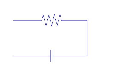
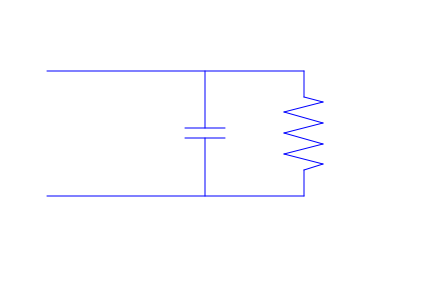
We can also plot a circuit where the resistor and capacitor are in parallel. All of the same techniques apply, we simply put the components in different locations. To do this, we type:
When we execute this, MuPAD gives us:


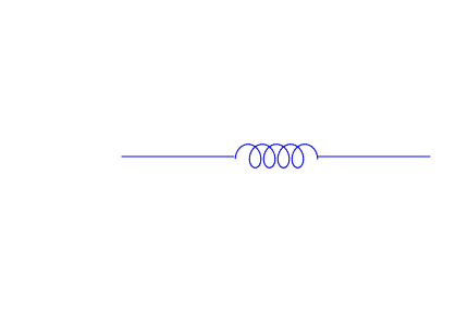
Sometimes we want to add inductors to our circuits. Instead of the linear curves that we plotted to get other components, we must use a parametric curve to create an inductor.

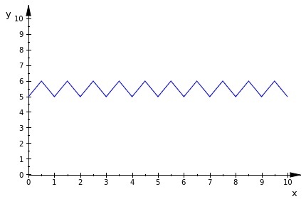
The following code is intended to be used in order to draw resistors in circuits. It is a triangular wave function, whose amplitude (a) and height (z) can easily be changed through parameters in the function. This resistor function makes use of the floor function, which rounds down to the nearest integer.

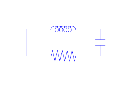
This is an example of a resistor in a circuit complete with a capacitor and inductor. Here, the amplitude is .5, the function is shifted up 5, and the domain of the resistor is [10,15].

 

Example. An inductor, also called a coil, is a passive two-terminal electrical component that consists of a conductor such as a wire, usually wound into a coil. When the current flowing through an inductor changes, the time-varying magnetic field induces a voltage in the conductor, that always opposes a change in current. The standard unit of inductance is the henry, abbreviated H. This is a large unit. More common units are the microhenry, abbreviated μH (1 μH = 10^-6H) and the millihenry, abbreviated mH (1 mH = 10^-3 H).

A capacitor is an electronic device that stores charge and energy. Capacitors can give off energy much faster than batteries can, giving them much higher power density than batteries with the same amount of energy. A capacitor holds very little energy compared to a battery, in general. It will smooth out short spikes in current, but will not help with longer bumps or continuous demand. Inductors are used with capacitors in various wireless communications applications. An inductor connected in series or parallel with a capacitor can provide discrimination against unwanted signals. Large inductors are used in the power supplies of electronic equipment of all types, including computers and their peripherals.

Consider an electric circuit, consisting of an inductor and capacitor, in series. To be more specific, assume that the capacitor is varied as a given function of time in a step wise fashion about its mean capacitance, C₀, by a small amount. The charge q(t) on the capacitor satisfies the linear ordinary differential equation with periodic coefficient (dot stands for the derivative with respect to time t):

Upon changing the independent variable to \( t' = \omega_0 t , \) where \( \omega_0^2 = 1 / \left( LC_0 \right) \) , the problem will be reduced to the following two ordinary differential equations with constant coefficients: that should be solved sequentially to satisfy countinuity conditions: at the points of discontuity the functions \( q_{\pm} \) should match each other including their first derivatives. Recall that we assume that \( 0 < \varepsilon < 1 . \) Now we formulate a sequence of initial value problems for charge q(t) in the circuit with periodically oscillated capacitor. For convenience, let us introduce two parameters: \( \omega^2_{+} = 1/\left( 1+ \varepsilon \right) \quad\mbox{and} \quad \omega^2_{-} = 1/\left( 1- \varepsilon \right) . \) Denoting the period 2T, we start with the initial value problem on the interval [0,T]: where Q is the initial charge. Solving this initial value problem on the interval [0,T], we obtain At t = T, the capacitor switches from ω_- to ω₊, and we get the initial value problem on the interval [T, 2T]: It has the unique solution Therefore, on the interval [0,2T], we have On next interval [2T, 3T], we have to solve the initial value problem for \( q_{2m} (t) \equiv q_{-} (t) \) and then for \( q_{2p} (t) \equiv q_{+} (t) \) We extend this process by switching from plus to minus on each interval of length 2T.