Linear Systems of Algebraic Equations
This page presents some topics from Linear Algebra needed for construction of solutions to systems of linear algebraic equations and some applications. We use matrices and vectors as essential elements in obtaining and expressing the solutions.
Matrices and Vectors
The central problem of linear algebra is to solve a linear system of equations. This means that the unknowns are only multiplied by numbers.
Our first example of a linear system has two equations in two unknowns:
\[
\begin{cases}
x-3y &= -1 , \\
2x+y &=5 .
\end{cases}
\]
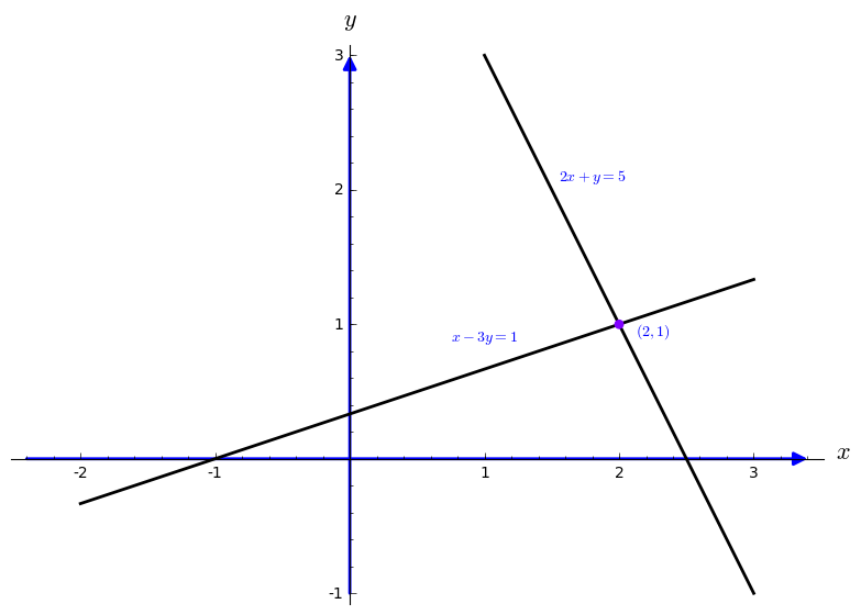
We begin with a row at a time. The first equation \( x-3y=-1 \) produces a straight line in the
\( xy- \) plane. The second equation \( 2x+y=5 \) defines another
line. By plotting these two lines, you cannot miss the intersection point where two lines meet. The point
\( x=2, \ y=1 \) lies on both lines. That point solves both equations at once.
Now we visualize this with a picture:
sage: l1=line([(-2,-1/3), (3,4/3)],thickness=2,color="black")
sage: l2=line([(1,3), (3,-1)],thickness=2,color="black")
sage: ah = arrow((-2.4,0), (3.4,0))
sage: av = arrow((0,-1), (0,3))
sage: P=circle((2.0,1.0),0.03, rgbcolor=hue(0.75), fill=True)
sage: t1=text(r"$(2,1)$",(2.25,0.95))
sage: t2=text(r"$x-3y=1$",(1.0,0.9))
sage: t2=text(r"$x-3y=1$",(1.0,0.9))
sage: t3=text(r"$2x+y=5$",(1.8,2.1))
sage: show(l1+l2+ah+av+t1+t2+t3+P,axes_labels=['$x$','$y$'])
Now we plot another graph:
sage: ah = arrow((-3.1,0), (2.2,0))
sage: av = arrow((0,-0.2), (0,5.1))
sage: a1=arrow([0,0],[-3,1], width=2, arrowsize=3,color="black")
sage: a2=arrow([0,0],[1,2], width=2, arrowsize=3,color="black")
sage: a3=arrow([0,0],[2,4], width=2, arrowsize=3,color="black")
sage: a4=arrow([0,0],[-1,5], width=2, arrowsize=3,color="black")
sage: l1=line([(-3,1), (-1,5)],color="blue",linestyle="dashed")
sage: l2=line([(2,4), (-1,5)],color="blue",linestyle="dashed")
sage: t1=text(r"${\bf v}_1$",(-3,0.85),color="black")
sage: t2=text(r"${\bf v}_2$",(1.1,1.85),color="black")
sage: t3=text(r"$2{\bf v}_2$",(2.05,3.75),color="black")
sage: t4=text(r"${\bf v}_1 + 2{\bf v}_2$",(-0.75,4.75),color="black")
sage: show(av+ah+a1+a2+a3+a4+l1+l2+t1+t2+t3+t4,axes_labels=['$x$','$y$'])
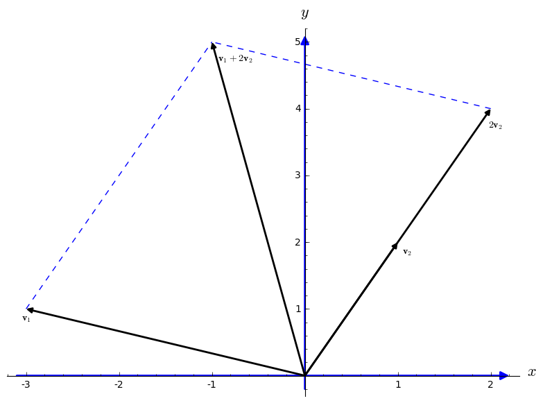
The row picture shows that two lines meet at a single point. Then we turn to the column picture by rewriting the system in vector form:
\[
x \begin{bmatrix}
1 \\
2
\end{bmatrix} + y \begin{bmatrix}
-3 \\
1
\end{bmatrix} = \begin{bmatrix}
-1 \\
5
\end{bmatrix} = {\bf b} .
\]
This has two columns on the left.
The problem is to find the combination of those vectors that equals the vector on the right.
We are multiplying the first column by \( x \) and the second by \( y ,\) and adding.
The figure at the right illustrates two basic operations with vectors: scalar multiplication and vector addition. With these two operations, we are able to build linear combination of vectors:
\[
2 \begin{bmatrix}
1 \\
2
\end{bmatrix} + 1 \begin{bmatrix}
-3 \\
1
\end{bmatrix} = \begin{bmatrix}
-1 \\
5
\end{bmatrix} .
\]
The
coefficient matrix on the left side of the equations is 2 by 2 matrix
A:
\[
{\bf A} = \begin{bmatrix}
1 & -3 \\
2 & 1
\end{bmatrix} .
\]
This allows us to rewrite the given system of linear equations in vector form (also sometimes called the matrix form, but we reserve the matrix form for matrix equations)
\[
{\bf A} \, {\bf x} = {\bf b} ,\qquad\mbox{which is }\quad \begin{bmatrix}
1 & -3 \\
2 & 1
\end{bmatrix} \, \begin{bmatrix}
x \\
y
\end{bmatrix} = \begin{bmatrix}
-1 \\
5
\end{bmatrix} .
\]
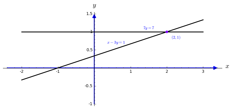
We use the above linear equation to demonstrate a great technique, called elimination. Before elimination,
\( x \)
and
\( y \) appear in both equations. After elimination, the first unknown
\( x \)
has disappeared from the second equation:
\[
{\bf Before: }\quad \begin{cases} x-3y &= -1 , \\
2x+y &=5 .
\end{cases} \qquad {\bf After: } \quad \begin{cases} x-3y &= -1 , \\
7\,y &=7
\end{cases} \qquad \begin{array}{l} \mbox{(multiply by 2 and subtract)} \\
(x \mbox{ has been eliminated).}
\end{array}
\]
The last equation
\( 7\,y =7 \) instantly gives
\( y=1. \) Substituting for
\( y \) in the first equation leaves
\( x -3 = -1. \) Therefore,
\( x=2 \) and the solution
\( (x,y) =(2,1) \) is complete.
sage: l1=line([(-2,-1/3), (3,4/3)],thickness=2,color="black")
sage: l2=line([(-2,1), (3,1)],thickness=2,color="black")
sage: ah = arrow((-2.4,0), (3.4,0))
sage: av = arrow((0,-1), (0,1.5))
sage: P=circle((2.0,1.0),0.03, rgbcolor=hue(0.75), fill=True)
sage: t1=text(r"$(2,1)$",(2.25,0.85))
sage: t2=text(r"$x-3y=1$",(0.6,0.7))
sage: t3=text(r"$7y=7$",(1.5,1.1))
sage: show(l1+l2+ah+av+t1+t2+t3+P,axes_labels=['$x$','$y$'])
A system of
\( m \) equations in
\( n \) unknowns
\( x_1 , \ x_2 , \ \ldots , \ x_n \) is a set of
\( m \) equations of the form
\[
\begin{cases}
a_{11} \,x_1 + a_{12}\, x_2 + \cdots + a_{1n}\, x_n &= b_1 ,
\\
a_{21} \,x_1 + a_{22}\, x_2 + \cdots + a_{2n}\, x_n &= b_2 ,
\\
\qquad \vdots & \qquad \vdots
\\
a_{m1} \,x_1 + a_{m2}\, x_2 + \cdots + a_{mn}\, x_n &= b_n .
\end{cases}
\]
The numbers
\( a_{ij} \) are known as the
coefficients of the system. The matrix
\( {\bf A} = [\,a_{ij}\,] , \) whose
\( (i,\, j) \) entry is the
coefficient
\( a_{ij} \) of the system of linear equations is called the coefficient matrix and is denoted by
\[
{\bf A} = \left[ \begin{array}{cccc} a_{1,1} & a_{1,2} & \cdots & a_{1,n} \\
a_{2,1} & a_{2,2} & \cdots & a_{2,n} \\
\vdots & \vdots & \ddots & \vdots \\
a_{m,1} & a_{m,2} & \cdots & a_{m,n} \end{array} \right] \qquad\mbox{or} \qquad {\bf A} = \left( \begin{array}{cccc} a_{1,1} & a_{1,2} & \cdots & a_{1,n} \\
a_{2,1} & a_{2,2} & \cdots & a_{2,n} \\
\vdots & \vdots & \ddots & \vdots \\
a_{m,1} & a_{m,2} & \cdots & a_{m,n} \end{array} \right) .
\]
Let
\( {\bf x} =\left[ x_1 , x_2 , \ldots x_n \right]^T \) be the vector of unknowns. Then the product
\( {\bf A}\,{\bf x} \) of the
\( m \times n \) coefficient matrix
A and the
\( n \times 1 \) column vector
x is an
\( m \times 1 \) matrix
\[
\left[ \begin{array}{cccc} a_{1,1} & a_{1,2} & \cdots & a_{1,n} \\
a_{2,1} & a_{2,2} & \cdots & a_{2,n} \\
\vdots & \vdots & \ddots & \vdots \\
a_{m,1} & a_{m,2} & \cdots & a_{m,n} \end{array} \right] \, \begin{bmatrix} x_1 \\ x_2 \\ \vdots \\ x_n \end{bmatrix}
= \begin{bmatrix} a_{1,1} x_1 + a_{1,2} x_2 + \cdots + a_{1,n} x_n
\\ a_{2,1} x_1 + a_{2,2} x_2 + \cdots + a_{2,n} x_n \\ \vdots \\ a_{m,1} x_1 + a_{m,2} x_2 + \cdots + a_{m,n} x_n \end{bmatrix} ,
\]
whose entries are the right-hand sides of our system of linear equations.
If we define another column vector \( {\bf b} = \left[ b_1 , b_2 , \ldots , b_m \right]^T \)
whose components are the right-hand sides \( b_{i} ,\) the system is equivalent to the vector equation
\[
{\bf A} \, {\bf x} = {\bf b} .
\]
We say that \( s_1 , \ s_2 , \ \ldots , \ s_n \) is a solution of the system if all
\( m \) equations hold true when
\[
x_1 = s_1 , \ x_2 = s_2 , \ \ldots , \ x_n = s_n .
\]
Sometimes a system of linear equations is known as a set of simultaneous equations; such terminology emphasises that a solution is an assignment of values to each of the
\( n \) unknowns such that each and every equation holds with this assignment. It is also referred to simply as a linear system.
Example. The linear system
\[
\begin{cases}
x_1 + x_2 + x_3 + x_4 + x_5 &= 3 ,
\\
2\,x_1 + x_2 + x_3 + x_4 + 2\, x_5 &= 4 ,
\\
x_1 - x_2 - x_3 + x_4 + x_5 &= 5 ,
\\
x_1 + x_4 + x_5 &= 4 ,
\end{cases}
\]
is an example of a system of four equations in five unknowns,
\( x_1 , \ x_2 , \ x_3 , \ x_4 , \ x_5 . \)
One solution of this system is
\[
x_1 = -1 , \ x_2 = -2 , \ x_3 =1, \ x_4 = 3 , \ x_5 = 2 ,
\]
as you can easily verify by substituting these values into the equations. Every equation is satisfied for these values of
\( x_1 , \ x_2 , \ x_3 , \ x_4 , \ x_5 . \)
However, there is not the only solution to this system of equations. There are many others.
On the other hand, the system of linear equations
\[
\begin{cases}
x_1 + x_2 + x_3 + x_4 + x_5 &= 3 ,
\\
2\,x_1 + x_2 + x_3 + x_4 + 2\, x_5 &= 4 ,
\\
x_1 - x_2 - x_3 + x_4 + x_5 &= 5 ,
\\
x_1 + x_4 + x_5 &= 6 ,
\end{cases}
\]
has no solution. There are no numbers we can assign to the unknowns
\( x_1 , \ x_2 , \ x_3 , \ x_4 , \ x_5 \) so that all four equations are satisfied. ■
In general, we say that a linear system of algebraic equations is consistent if it has at least one solution and inconsistent if it has no solution. Thus, a consistent linear system has either one solution or infinitely many solutions---there are no other possibilities.
Theorem: Let A be an \( m \times n \) matrix.
-
(Overdetermined case) If m > n, then the linear system \( {\bf A}\,{\bf x} = {\bf b} \)
is inconsistent for at least one vector b in \( \mathbb{R}^n . \)
- (Underdetermined case) If m < n, then for each vector b in \( \mathbb{R}^m \)
the linear system \( {\bf A}\,{\bf x} = {\bf b} \) is either inconsistent or has infinite many solutions.
Theorem: If A is an \( m \times n \) matrix with
\( m < n, \) then \( {\bf A}\,{\bf x} = {\bf 0} \) has
infinitely many solutions.
Theorem: A system of linear equations \( {\bf A}\,{\bf x} = {\bf b} \) is consistent if and only if b is in the column space of A.
Theorem: A linear system of algebraic equations \( {\bf A}\,{\bf x} = {\bf b} \) is consistent if and only if the vector b is orthogonal
to every solution y of the adjoint homogeneous equation \( {\bf A}^T \,{\bf y} = {\bf 0} \) or \( {\bf y}^T {\bf A} = {\bf 0} . \) ■
Sage uses standard commands to solve linear systems of algebraic equations:
\[
{\bf A} \, {\bf x} = {\bf b} .
\]
Here A is m-by-n matrix, b is a given vector of size m and column-vector x of size n is to be determined. An augmented matrix is a matrix
obtained by appending the columns of two given matrices, usually for the purpose of performing the same elementary row operations on each of the given matrices.
We associate with the given system of linear equations \( {\bf A}\,{\bf x} = {\bf b} \) an augmented matrix by appending the column-vector b to the matrix A.
Such matrix is denoted by \( {\bf M} = \left( {\bf A}\,\vert \,{\bf b} \right) \) or \( {\bf M} = \left[ {\bf A}\,\vert \,{\bf b} \right] : \)
\[
{\bf M} = \left( {\bf A}\,\vert \,{\bf b} \right) = \left[ {\bf A}\,\vert \,{\bf b} \right] =
\left[ \begin{array}{cccc|c} a_{1,1} & a_{1,2} & \cdots & a_{1,n} & b_1 \\
a_{2,1} & a_{2,2} & \cdots & a_{2,n} & b_2 \\
\vdots & \vdots & \ddots & \vdots & \vdots\\
a_{m,1} & a_{m,2} & \cdots & a_{m,n} & b_m \end{array} \right] .
\]
Theorem: Let A be an \( m \times n \) matrix. A linear system of equations
\( {\bf A}\,{\bf x} = {\bf b} \) is consistent if and only if the rank of the coefficient matrice A is the same as the rank of the augmented matrix \( \left[ {\bf A}\,\vert \, {\bf b} \right] . \) ■
The actual use of the term augmented matrix appears to have been introduced by the American mathematician Maxime Bocher (1867--1918) in 1907.
We show how it works by examples. The system can be solved using solve command
sage: solve([eq1==0,eq2==0],x1,x2)
However, this is somewhat complex and we use vector approach:
sage: A = Matrix([[1,2,3],[3,2,1],[1,1,1]])
sage: b = vector([0, -4, -1])
sage: x = A.solve_right(b)
sage: x
(-2, 1, 0)
sage: A * x   # checking our answer...
(0, -4, -1)
A backslash \ can be used in the place of solve_right; use
A \ b instead of A.solve_right(b).
If there is no solution, Sage returns an error:
sage: A.solve_right(w)
Traceback (most recent call last):
...
ValueError: matrix equation has no solutions
Similarly, use A.solve_left(b) to solve for row-vector x in
\( {\bf x}\, {\bf A} = {\bf b}\), which is equivalent to \( {\bf A}\,{\bf x} = {\bf b}^{\mathrm T} . \)
If a square matrix is nonsingular (invertible), then solutions of the vector equation \( {\bf A}^{\mathrm T} {\bf x}^{\mathrm T} = {\bf b} \)
can be obtained by applying the inverse matrix:
\( {\bf x} = {\bf A}^{-1} {\bf b} . \) We will discuss this method later in the section devoted to inverse matrices.
Square Matrices
A very important class of matrices constitute so called square matrices that have the same number of rows as columns. In computer graphics, square matrices are used for transformations.
An n-by-n matrix is known as a square matrix of order n. Square matrices of the same order can be not only added, subtructed or multiplied by a constant, but also multiplied.
Theorem: If A is an \( n \times n \) matrix, then the following statements are equivalent.
-
A is invertible.
- \( {\bf A}\,{\bf x} = {\bf 0} \) has only the trivial solution.
-
The reduced row echelon form (upon application of Gauss--Jordan elimination) is the identity matrix.
- A has nullity/kernel 0.
- A has rank n.
- A is expressible as a product of elementary matrices.
- \( {\bf A}\,{\bf x} = {\bf b} \) is consistent for every \( n \times 1 \) matrix b (column vector).
- \( {\bf A}\,{\bf x} = {\bf b} \) has exactly one solution for every \( n \times 1 \) matrix b.
- \( \det ({\bf A} ) \ne 0 .\)
- \( \lambda =0 \) is not an eigenvalue of A.
- The row vectors of A span \( \mathbb{R}^n . \)
- The column vectors of A form a basis for \( \mathbb{R}^n . \)
Theorem: If A is an invertible matrix, then A AT
and ATA are also invertible.
To view this, type show(P+Q+R).
Numerical Methods
The condition number of an invertible matrix
A is defined to be
\[
\kappa ({\bf A}) = \| {\bf A} \| \, \| {\bf A}^{-1} \| .
\]
This quantity is always bigger than (or equal to) 1.
We must use the same norm twice on the right-hand side of the above equation. Sometimes the
notation is adjusted to make it clear which norm is being used, for example if we use the infinity
norm we might write
\[
\kappa_{\infty} ({\bf A}) = \| {\bf A} \|_{\infty} \, \| {\bf A}^{-1} \|_{\infty} .
\]
Inequalities
Regarding
Applications
- into \(N\)
subintervals,
- the approximation given by the Riemann sum approximation.
sage: f1(x) = x^2
sage: f2(x) = 5-x^2
sage: f = Piecewise([[(0,1),f1],[(1,2),f2]])
sage: f.trapezoid(4)
Piecewise defined function with 4 parts, [[(0, 1/2), 1/2*x],
[(1/2, 1), 9/2*x - 2], [(1, 3/2), 1/2*x + 2],
[(3/2, 2), -7/2*x + 8]]
sage: f.riemann_sum_integral_approximation(6,mode="right")
19/6
sage: f.integral()
Piecewise defined function with 2 parts,
[[(0, 1), x |--> 1/3*x^3], [(1, 2), x |--> -1/3*x^3 + 5*x - 13/3]]
sage: f.integral(definite=True)
3