

3D plotting
We show how to plot a function of two variables by examples.
|
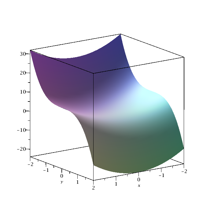
plot3d(2*x^2-3*y^3,x=-2..2,y=-2..2);
In its most basic form, the plot3d command takes three arguments. The first is the expression that defines the function to be plotted, and the next two are the ranges of the independent variables. |
|
| Figure 1: 3dplot. | Maple code |
Note: To see a different view, use the mouse to click and drag in the plot. To change some of the plot options, right-click on the plot, and select an option. For example, try using the mouse to add axes to the plot.
Just like the plot command, the plot3d command can be given many optional arguments. Look for plot3d in the Maple Help, or enter the command ?plot3d to learn more. Here is a similar command as above, with some options added directly to the command.
|
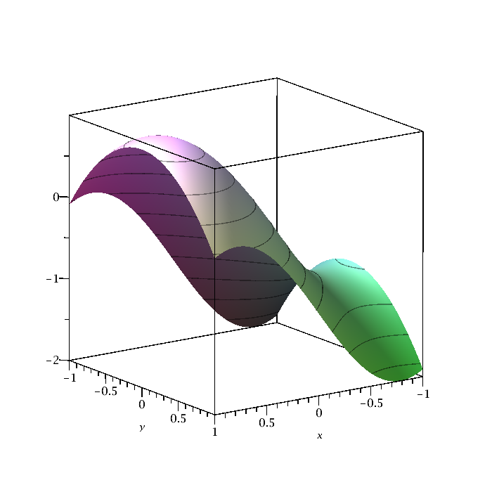
plot3d(sin(2*x)-y^2,x=-1..1,y=-1..1,axes=boxed,grid=[64,64],style=patchcontour);
There are many other options. With the "style=patchcontour" option, the lines drawn in the surface are contours lines instead of the xy grid. If you look at the plot "from above'', you will see the contour diagram |
|
| Figure 2: 3dplot with options. | Maple code |
|
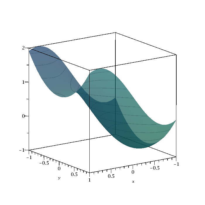
plot3d(sin(2*x)+y^2,x=-1..1,y=-1..1,ambientlight=[0.1, 0.5, 0.4],transparency=0.5,axes=boxed,style=patchcontour);
There are many other options. |
|
| Figure 3: 3dplot with options. | Maple code |
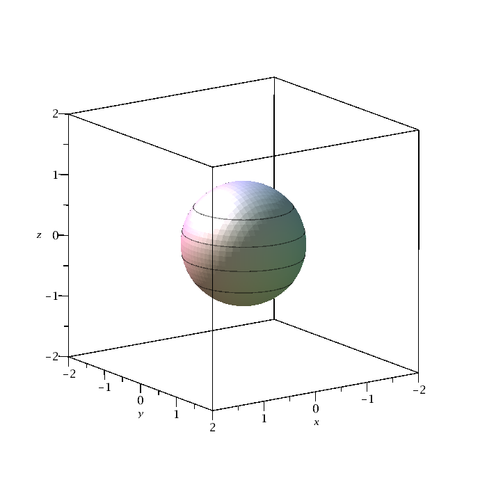
A surface can be defined implicitly, rather than as the graph of a function of two variables. That is, instead of defining the surface as z = f(x, y), it may be defined as a level set g(x, y, z) = C. There is a command in Maple, called
implicitplot3d that can be used to plot such surfaces. To use it, we must first load a library of functions with the with(plots): command. (Don't worry about the warning that appears after this command is entered.)
|
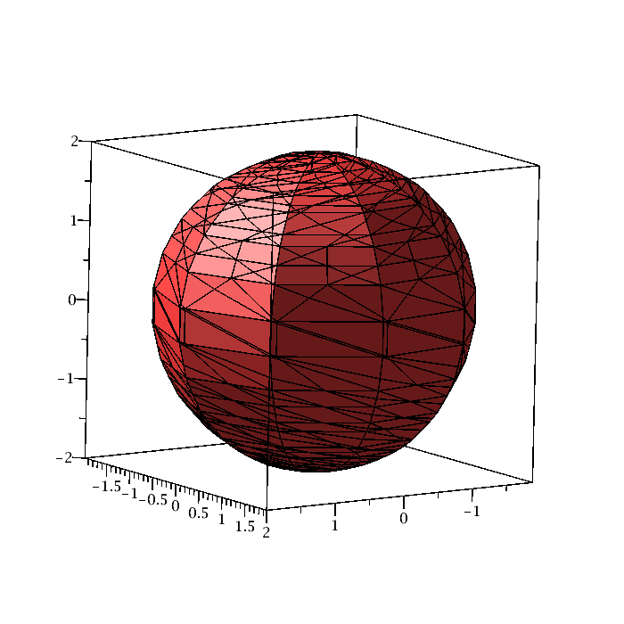
with(plots): implicitplot3d(x^2+y^2+z^2=1,x=-2..2,y=-2..2,z=-2..2,grid=[50,50,50],style=patchcontour,scaling=constrained,axes=boxed); There are many other options. |
|
| Figure 4: Implicit plot. | Maple code |
|
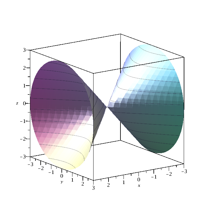
with(plots): implicitplot3d(x^2=y^2+z^2,x=-3..3,y=-3..3,z=-3..3,grid=[25,25,25],style=patchcontour,scaling=constrained); There are many other options. |
|
| Figure 5: Implicit plot. | Maple code |
|
with(plots): implicitplot3d( z^2 +r^2 =4, r=0..2, theta=0..2*Pi, z=-2..2, coords=cylindrical,color=orange) There are many other options. |
|
| Figure 6: Implicit plot in cylindrical coordinates. | Maple code |
Example:
**DESCRIPTION OF PROBLEM GOES HERE**
This is a description for some Maple code. Maple is an extremely
useful tool for many different areas in engineering, applied
mathematics, computer science, biology, chemistry, and so much
more. It is quite amazing at handling matrices, but has lots of
competition with other programs such as Mathematica and Maple. Here is
a code snippet plotting two lines (y vs. x and z vs. x)
on the same graph:
(a*b)/c+13*d
ur code
another line
\[ {\frac {ab}{c}}+13\,d \]
- Reference 1
- Reference 2