An inverted pendulum is not stable. Nevertheless, as pointed out by Pyotr Kapitza (1894--1984) in 1951, if you oscillate vertically the suspension point at a sufficientlyfast frequency Ω, you can stabilise it.
A similar phenomenon occurs in arotating saddle (see video), and is also used to create radio-frequencyionic traps.
Let us start considering a very familiar one-dimensional system: a planar pendulum made of a massless rod of length ℓ ending with a point mass m. In the familiar swing, the driving occurs in different ways: if you “drive” the swing yourself, you do it by effectively modifyingthe position of your “center-of-mass”, hence the effective length ℓ(t) of the “pendulum”. If you are pushed by someone else, then you have a pendulum with a “periodic external force”.
We use the generalize coordinate q = θ that denotes the angle formed with the vertical (θ = 0 being the
downward position), and y0(t) denotes the position of its suspension point, we can derive the equations of motion from the Lagrangian formalism. In a short while we will assume that y0(t) = Acos Ωt, where A is the amplitude of the driving and Ω the driving frequency, but for the time being, let us proceed by keeping y0(t to be general. In a system of reference with the y-axis oriented upwards and the x-axis horizontally, the position x(t) and y(t) of the massm is:
where we dropped the term \( \frac{m}{2}\,\dot{y}_0^2 - mgy_0 \) because it would not enter in the Euler--Lagrange equations due to pure dependence on time t. The associated momentum is given by:
where \( \omega_0^2 = g/\ell \) is the square of
the frequency of the unperturbed pendulum in the linear regime, Ω is the driving frequency, A is the amplitude of the driving, which we model as y0(t) = Acos(Ωt).
Example 1:
If a rod or a pencil is held upright on a table, and then released, it will fall onto the ground. We consider a simple case when a rigid rod of length 2ℓ is fixed to a horizontal table by a smooth hinge at one end while another end is free to fall.
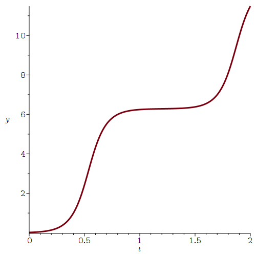
Let us plot the solution of the pendulum equation: