Sturm--Liouville theory is actually a generalization for the infinite dimensional case of famous
eigenvalue/eigenvector problems for finite square matrices that we discussed in Part I of this tutorial. Although a Sturm--Liouville problem can be
formulated in operator form as L[ y ] = λy similar to the matrix eigenvalue
problem Ax = λx, where the operator L is an unbounded differential
operator and y is a smooth function.
The corresponding theory that is known as Sturm--Liouville theory originated in two articles by the French
mathematician of German descent Jacques Charles François Sturm
(1803--1855).
Sturm, J.C.F.,
"Mémoire sur les Équations différentielles linéaires du second ordre",
Journal de Mathématiques Pures et Appliquées, 1836, Vol. 1,
pp. 106-186. [sept. 28, 1833]
Sturm, , J.C.F.,
"Mémoire sur une classe des d'Équations à différences partielles".
Journal de Mathématiques Pures et Appliquées, 1836, Vol. 1,
pp. 373--444.
Following the same 1836 year, Sturm together with his friend, the
French
mathematician Joseph
Liouville (1809--1882), published very influential articles that provided crucial groundwork for the
theory.
Sturm & Liouville,
"Démonstration d'un théorème de M. Cauchy relatif aux racines imaginaires des
équations".
Journal de Mathématiques Pures et Appliquées, 1836, Vol. 1,
pp. 278--289.
Sturm & Liouville,
"Note sur un théorème de M. Cauchy relatif aux racines des équations
simultanées", Comptes rendus de l'Académie des Sciences (English: Proceedings of the
Academy of Sciences), 1837, Vol. 4, pp. 720--739.
Sturm & Liouville,
"Extrait d'un Mémoire sur le développement des fonctions en séries dont les
différents termes sont assujettis à satisfaire à une même équation
différentielle lindaire, contenant un paramètre variable",
Journal de Mathématiques Pures et Appliquées, 1837, Vol 2,
pp. 220--233.
Comptes rendus de l'Académie des Sciences ((English: Proceedings of the Academy of sciences),
1837, Vol. 4, pp. 675--677.
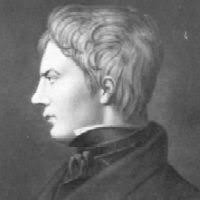
Jacques Sturm
A classical Sturm–Liouville theory,
named after Jacques Charles
François Sturm (1803--1855) and Joseph
Liouville (1809--1882),
involves analysis of eigenvalues and eigenfunctions for a second order
linear differential operator (we use letter L to emphasize that this is a linear operator)
where I is the identity operator, and p(x) and q(x) are given continuous
functions on some interval [𝑎, b]. Since p(x) follows the derivative operator, it
should be a differentiable function. The linear self-adjoint operator \eqref{EqSturm.3} is referred to as the
Sturm--Liouville operator.
Correspondingly, the Sturm--Liouville
theory is about a real second-order homogeneous linear self-adjoint differential equation with a parameter
λ of the form
\begin{equation} \label{EqSturm.1}
\frac{\text d}{{\text d}x} \left[ p(x)\,\frac{{\text d}y}{{\text d}x}
\right] - q(x)\, y + \lambda \,\rho (x)\,y(x) =0 , \qquad a < x < b ,
\end{equation}
Here y = y(x) is a nontrivial (meaning not identically zero) function of the free variable
x∈[𝑎, b]. A positive function ρ(x) is called the "weight" or "density"
function---it is not a part of the differential operator \eqref{EqSturm.3}. On the other hand,
functions p(x), p'(x), and q(x) are specified at the outset. In the
simplest of cases, all coefficients are continuous on the finite closed interval [𝑎, b], and
p(x) has continuous derivative. In this simplest case, a nontrivial function y(x) is
called a solution of Eq.\eqref{EqSturm.1} if it is twice continuously differentiable on (𝑎, b)
and satisfies the given equation at every point in (𝑎, b).
Let us consider an arbitrary second order differential equation
\[
M\left[ x, \texttt{D} \right] u = a(x)\,u'' + b(x)\, u' + c(x)\, u = 0 ,
\]
with some given continuous functions 𝑎(x), b(x), and c(x). We
denote by p(x) an integrating factor
we can rewrite this Sturm--Liouville problem in operator form:
\begin{equation} \label{EqSturm.5}
L\left[ x, \texttt{D} \right] y = \rho\,\lambda y , \qquad B_a y = 0, \quad B_{b} y = 0.
\end{equation}
This boundary value problem has an obvious solution---the identically zero function. Since we are not after such
a trivial solution, we need something more. The Sturm--Liouville problem (S-L, for short) consists of two
parts: the first part is about finding values of parameter λ for which the problem has a nontrivial
solution (not identically zero); such values are called eigenvalues. The second part includes
determination of nontrivial solutions that are called eigenfunctions. Note that a Sturm--Liouville
problem may have other constraints, not necessarily formulated above.
There are two kinds of Sturm--Liouville problems. One is called classical or regular when
p(x) > 0 and 1/p(x) > 0 for all points from the closed interval
x∈[𝑎, b]. These assumptions are necessary to render the theory as simple as
possible while retaining considerable generality. It turns out that these conditions are valid in many
problems that we will consider shortly. If p(𝑎) = 0, or p(b) = 0, or
p(𝑎) = 0 = p(b), the Sturm--Liouville problem is said to be singular. If
conditions on coefficients p(x), q(x), and ρ(x) are held to make the
Sturm--Liouville problem regular, but the interval is unbounded, then such problem is also referred to as
singular.
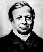
Joseph Liouville
Jacques Charles François Sturm (1803--1855) was a French mathematician of Switzerland descent. Charles spent
his adult life in Paris. His primary interests were fluid mechanics and differential equations. Sturm along
with the Swiss engineer Daniel Colladon was the first to accurately determine the speed of sound in water. In
mathematics, he won the coveted Grand prix des Scienes Mathematiques for his work in differential equations.
Sturm held the chair of mechanics at the Sorbonne and was elected a member of the French Academy of Sciences. The asteroid
31043 Sturm is named for him. Sturm's name is one of the 72 names engraved at the Eiffel Tower.
Joseph Liouville was a French mathematician known for his work in analysis, differential geometry, and
number theory and for his discovery of transcendental numbers---i.e., numbers that are not the roots of
algebraic equations having rational coefficients. He was also influential as a journal editor and teacher.
Joseph founded the Journal de
Mathématiques Pures et Appliquées which retains its high reputation up to today.
In physics and other applications, many problems arise in the form of boundary
value problems involving second order ordinary differential equations, written
in self-adjoint form:
where \( \texttt{D} = {\text d}/{\text d}x \) is
the derivative operator and \( \texttt{I} = \texttt{D}^0 \) is the identity
operator. Sturm was the first who generalized the well known
matrix problem for eigenvalues/eigenvectors to the linear differential
operators by considering the eigenvalue problem \eqref{EqSturm.5}
for functions y(x) subject to some boundary conditions. Now this problem is referred to as the
Sturm--Liouville problem.
Here p(x), q(x), and ρ(x) > 0 are specified continuous functions at
the outset, which is usually some interval (finite or not) of real axis ℝ.
Example 1:
Let us consider the Sturm--Liouville problem with periodic boundary conditions
Solutions of the differential equation \( y'' + \lambda \,y =0 \) depend on the
sign of parameter λ. If λ = -μ2 is negative, the equation has two exponential
linearly independent solutions \( y_1 = e^{\mu x} \quad\mbox{and}\quad y_2 = e^{-\mu x}
\) that also sometimes can be written through hyperbolic sine and cosine functions. These
functions cannot be periodic, so negative λ is not an eigenvalue.
If λ = 0, the general solution of the differential equation \( y'' =0 \)
is a linear function \( y = a + b\,x , \) which could be periodic only when
b = 0. So zero is an eigenvalue corresponding to an eigenfunction which is a constant function in
this case.
If λ = μ2 is positive, then the general solution becomes
\[
y = a\,\cos (\mu x) + b\,\sin (\mu x) ,
\]
with some constants 𝑎 and b. This function is periodic with period T if and only if
μ is proportional to 2π/T; so we get eigenvalues
with some real constants 𝑎n, bn. These arbitrary constants indicate
that the eigenfunction is two-dimensional. Of course, you can organize it in one-dimensional array upon
introducing positive and negative indices:
When a function is specified at the boundary, then the corresponding boundary conditions are named after G. Dirichlet.
Solutions of the differential equation \( y'' + \lambda \,y =0 \) depend on the
sign of parameter λ. If λ = -μ2 is negative, the equation has two exponential
linearly independent solutions \( y_1 = e^{\mu x} \quad\mbox{and}\quad y_2 = e^{-\mu x} .
\)
Then the general solution becomes
\[
y(x) = c_1 e^{\mu x} + c_2 e^{-\mu x} ,
\]
with some constants c1 and c2. From the first boundary condition, we
have
It could be shown similarly to the previous example that negative λ are not possible. So we need to
consider only two cases: λ = 0 and λ = μ² > 0. The former gives us an eigenvalue
λ = 0 to which corresponds a constant as an eigenfunction. To the latter corresponds the general
solution
Example 4:
There are two known Sturm--Liouville problems with mixed boundary conditions when on one end we have the
Dirichlet condition while on the other end we have the Neumann condition. So we start with one of them:
with some constant c. It is clear from our previous discussion that eigenvalues must be positive in
this case. The Neumann condition at the right end dictates
When a product is zero then at least one multiple must be zero. Obviously, c cannot be zero,
otherwise we will have a trivial solution. Since λ > 0 according to assumption, we get the
condition
The transcendent equation (5.2) could be solved only by a numerical procedure such as Newton's method.
Nevertheless, if we let \( t = \sqrt{\lambda} , \) then we see from their graphs
that there exists an infinite number of roots of \( \tan t = -t . \)
Since tangent function has vertical asymptotes at \( t = \frac{\pi}{2} + n\pi , \quad
n=0,1,2,\ldots ; \) the roots tn of the equation \( \tan t =
-t \) approach
Charles Sturm was the first person who made a qualitative analysis of solutions to ordinary differential
equations with variable coefficients without any knowledge about these solutions; moreover, there were no
example of such solutions available at his time. To make appropriate analysis of solutions, we need to
introduce some function spaces of integrable functions that were invented by a Hungarian mathematician (of
Jewish descent) Frigyes Riesz in 1910. Actually, we
will use only three of them: C([𝑎, b]) ⊂ 𝔏² ⊂ 𝔏¹.
To prepare the ground for the Sturm–Liouville theory we survey basic function spaces.
To be more specific, we denote by 𝔏¹([𝑎, b], ρ) the set of (Lebesgue) integrable functions of the finite
norm
To simplify the
notation, sometimes this space is also denoted as 𝔏([𝑎, b], ρ) by dropping "1".
So a sequence of functions { fn(x) } converges in mean (or 𝔏¹) to
f(x) iff
Let f be a real- or complex-valued function defined on [𝑎, b] except, possibly, for
finitely many points. f is called piecewise continuous on [𝑎, b] if it has at
most
finitely many points of discontinuity, and if at any such point f admits left and right
limits (such a discontinuity is called a jump (or step) discontinuity).
Our next space, C([𝑎, b]), is also a Banach space; it consists of all real-valued
continuous functions on the closed interval [𝑎, b] with the norm
There is no standard notation for inner product: in mathematics, it is common to separate functions f
and g by a comma, while in physics, they are usually separated by a vertical line. We utilize both
notations in hope to confuse the reader. Also, a complex conjugate \( \overline{f(x)} \)
of the function f(x) is usually denoted in mathematics by overline. Physicists prefer to
use asterisk for complex conjugate.
is called the characteristic function of the interval [α, β].
The sequence of functions \( \displaystyle \phi_n = \chi_{[n , n+1 ]} (x) , \quad
n=1,2,3,\ldots , \) converges pointwise to zero on [0, ∞), but \(
\displaystyle \| \phi_n \| = 1, \) so this sequence does not converge in norm to zero.
On the other hand, consider the interval [0, 1], and let {[𝑎n , bn]}
be a sequence
of intervals such that each x ∈ [0, 1] belongs, and also does not belong, to
infinitely many intervals [𝑎n , bn], and such that
bn − 𝑎n = 2 −k(n), where {k(n)} is a
nondecreasing sequence satisfying
\( \displaystyle \lim_{n\to\infty} k(n) = \infty . \) Since
it follows that the sequence { χ[𝑎n, bn] } tends to zero
function in the mean. However,
{ χ[𝑎n, bn] } does not converge at any point of [0, 1]
since for a fixed 0 ≤ x0 ≤ 1, the sequence { χ[𝑎n,
bn] } attains infinitely many times the value 0 and also infinitely many times the
value 1.
where L is the self-adjoint differential operator \eqref{EqSturm.3}.
Theorem 1: Properties of the regular Sturm--Liouville problem \eqref{EqSturm.1},
\eqref{EqSturm.2}.
Suppose that functions p(x), p'(x), q(x), ρ(x) are
continuous on [𝑎, b], and also p(x) and ρ(x) are positive. Then the
Sturm–Liouville problem \eqref{EqSturm.5} has the following properties.
There exists an infinite number of real eigenvalues that can be arranged in increasing order
λ1 < λ2 < λ3 < …
λn < … such that λn →∞ as
n→∞.
For each eigenvalue there is only one eigenfunction (up until nonzero
multiple).
Eigenfunctions corresponding to different eigenvalues are linearly
independent.
The set of eigenfunctions { ϕn } corresponding to the set of eigenvalues is
orthogonal with respect to the weight function ρ(x) on the interval x ∈ [𝑎,
b]:
Since λ ≠ μ, we obtain orthogonality of eigenfunctions ψ and φ.
Theorem 2:
If in addition to conditions of the previous statement, q(x) ≥ 0 and all coefficients
α0, α1, β0, β1 ≥ 0, then all
eigenvalues of Sturm--Liouville problem \eqref{EqSturm.5} are not negative.
When zero is an eigenvalue, we usually start labeling the eigenvalues at 0 rather than at 1 for convenience.
That is we label the eigenvalues 0 = λ0 < λ1 <
λ2 < ··· .
.
Sturm’s Comparison Theorem:
For i = 1,2, let ui(x) be a nontrivial solution of the differential equation
\( \displaystyle \left( p_i(x)\, u'_i \right)' + q_i u_i = 0 \) on α ≤
x ≤ β. Suppose further that the coefficients are continuous and for x ∈ [α,
β]
Then if α, β are two consecutive zeros of u1(x), the open interval
(α, β) will contain at least one zero of u2(x).
Sturm’s proofs of course do not meet the standards of modern rigor. They meet
the standards of his time, and are in fact correct in method and can without too
much trouble be made rigorous. The first efforts to do this are due to Maxime Bôcher
in a series of papers in the Bulletin of the AMS and are also contained in
his book. Bôcher remarks that “the work of Sturm may, however, be
made perfectly rigorous without serious trouble and with no real modification of
method”. The conditions placed on the coefficients were to make them piecewise
continuous. Bôcher used Riccati equation
techniques in some of his proofs; it should be noted
that Sturm mentions the Riccati equation, but does not employ it in his proofs.
Riccati equation techniques in variational theory go back at least to Legendre who
in 1786 gave a flawed proof of his necessary condition for a minimizer of an integral
functional. A correct proof of Legendre’s condition using Riccati equations can be
found in Bolza’s 1904 lecture notes. Bolza attributes this proof to Weierstrass.
Bôcher. M., The theorems of oscillation of Sturm and Klein, Bull. Amer. Math. Soc.
4 (1897–1898), 295–313, 365–376.
Bôcher, M., Leçons sur les méethodes de Sturm dans la théorie des équations
différentielles linéaires, et leurs déeveloppements modernes, Gauthier-Villars,
Paris, 1917.
Bolza, O., Lectures on the Calculus of Variations, Dover, New York, 1961.
Sturm’s Separation Theorem:
If u1(x), u2(x) are two linearly independent solutions of
the differential equation \( \displaystyle \left( p(x)\, u' \right)' + q\, u_i = 0 \)
and α, β are two consecutive zeros of u1(x), then
u2(x) has a zero on the open interval (α, β).
Theorem 5: Fredholm alternative.
Suppose that we have a regular Sturm–Liouville problem \eqref{EqSturm.5}. Then either the homogeneous
boundary value problem
Now we are going to take advantage of considering the differential operator \eqref{EqSturm.3} in the Hilbert
space 𝔏²([𝑎, b], ρ). First, using integration by parts, it is not hard to show
that the linear operator \eqref{EqSturm.3} is self-adjoint:
\[
\left\langle L \left[ x, \texttt{D} \right] u \,\vert \,v(x) \right\rangle = \int_a^b \left( \frac{{\text
d}}{{\text d}x}\,p(x)\, \frac{{\text d}u}{{\text d}x} - q(x)\,u(x) \right) v(x)\,\rho (x)\,{\text d}x =
\left\langle u\,\vert L \left[ x, \texttt{D} \right] v \right\rangle .
\]
However, the most important is the ability to compute the eigenfunction decomposition (which is actually the
spectral decomposition according to the differential operator L) of a wide class of functions. That is,
for any function f(x) ∈ 𝔏²([𝑎, b], ρ) satisfying the
prescribed boundary conditions, we wish to synthesize it as
where ϕk(x) are eigenfunctions. We wish to find out whether we can represent a
function in this way, and if so, we wish to calculate ck
(and of course we would want to know if the sum converges).
Although this topic will be considered in detail in a dedicated section. we
outline the main ideas.
Assuming that series \eqref{EqSturm.6} converges, we multiply it by an eigenfunction
ρ(x) ϕn(x) and integrate with respect to x from
𝑎 to b. This yields
These Fourier coefficients \eqref{EqSturm.8} satisfy the so-called Bessel inequality:
\[
\sum_{k\ge 1} \left\vert c_k \right\vert^2 \le \left\langle f , f
\right\rangle .
\]
A set of orthogonal functions {
φk } in 𝔏² is called complete in the closed
interval [𝑎,b]
whenever the vanishing of inner products with all the orthogonal functions implies the member of
𝔏²([𝑎, b], ρ) is equal to zero almost everywhere in the domain.
The term complete was introduced by the famous Russian mathematician
Vladimir Steklov
(1864--1926). A set of functions { φk } in 𝔏² is complete if and only if the Parseval identity holds:
The identity above was stated by the famous French mathematician Marc-Antoine Parseval (1755--1836) in 1799.
The main reason to study Sturn--Liouville problems is that their eigenfunctions
provide a basis for expansion for certain class of functions.
This tells us that basis functions have close relationships with
linear operators, and this basis is orthogonal for self-adjoint second order
differential operators. In other words, solutions of differential equations
can be approximated more efficiently by means of better basis functions. For
example, a periodic function or solution is expressed more efficiently
by periodic basis functions than by polynomials like the Taylor series.
For example, the linear operator
\( L\left[ y \right] = y'' + \lambda \,y \)
determines the basis functions. When λ < 0, the basis functions
will be
Decomposition of complicated systems into its constituent parts is one of science’s most powerful strategies
for analysis and understanding. Large-scale systems with linearly coupled components.
Spectral decomposition—splitting a linear operator into independent modes of simple behavior—is greatly
appreciated in mathematical physics.
For example, a wave dynamics is usually captured by superposition of simple modes.
Quantum mechanics and statistical mechanics identify the energy eigenvalues of Hamiltonians as the basic
objects in thermodynamics: transitions among the energy eigenstates yield heat and work. The eigenvalue
spectrum reveals itself most directly in other kinds of spectra, such as the frequency spectra of light
emitted by the gases that permeate the galactic filaments of our universe.
Spectral decomposition often allows a problem to be simplified by approximations that use only the dominant
contributing modes. Indeed, human-face recognition can be efficiently accomplished using a small basis of
“eigenfaces”. Certainly, there are many applications that highlight the importance of decomposition. In this
section, we concentrate our attention on application of decomposition theory to differential equations
generated by a linear second order self-adjoint operator subject to boundary conditions. Now it is known
that depending on boundary conditions, the corresponding boundary value problem may have discrete spectum
(set of eigenvalues) or continuous spectrum or their combination.
When solving an inhomogeneous differential equation
\[
L \left[ x, \texttt{D} \right] y = f ,
\]
with a differential operatoe L, we expand the input function and the unknown solution into the series
over eigenfunctions:
Titchmarsh, E.C., Eigenfunction expansions associated with second-order differential equations I,
Clarendon Press, Oxford, 1962.
Whittaker, E.T. and Watson, G.N., Modern analysis, Cambridge University Press, 1950
Zettl, A., Computing continuous spectrum, in Trends and Developments in Ordinary Differential Equations,
393–406, Y. Alavi and P. Hsieh editors, World Scientific, 1994.
Zettl, A., Sturm-Liouville problems, in Spectral Theory and
Computational Methods of Sturm-Liouville problems, 1–104, Lecture
Notes in Pure and Applied Mathematics 191, Marcel Dekker, Inc., New
York, 1997.