Mechanical Applications in MuPADBrown University Applied Mathematics |
Plotting solutions to differential equations can be useful in not only math classes, but in a number of disciplines. Differential equations are used to model scenarios in mechanics, electricity and magnetism, neuroscience, ecology, and much more. In this section, we present some application in Mechanics.
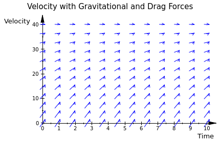
Example: When an object in free fall is being acted on by only the forces of air resistance (or some other fluid drag) and gravity, a differential equation can be written relating the acceleration to the velocity and two other constants describing these forces. For objects falling on earth, this equation is:
plot(field, Header="Velocity with Gravitational and Drag Forces", AxesTitles=["Time","Velocity"]):
This is nice, because in 2 lines of code, you can get a perfectly good direction field to your exact specifications.
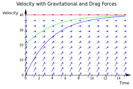
If we want to see how an object will approach terminal velocity (g=kv) based on its starting velocity, we can plot solution curves to the differential equation, as we have done in the past. The following plot shows the streamlines describing velocity as
acceleration := (x,y) -> [10-0.25*y[1]]:
solution1 := numeric::odesolve2(acceleration, 0, [0]):
curve1 := plot::Function2d(solution1(x)[1], x=0..xmax, LineColor = RGB::Blue):
solution2 := numeric::odesolve2(acceleration, 0, [20]):
curve2 := plot::Function2d(solution2(x)[1], x=0..xmax, LineColor = RGB::Green):
solution3 := numeric::odesolve2(acceleration, 0, [40]):
curve3 := plot::Function2d(solution3(x)[1], x=0..xmax, LineColor = RGB::Red):
plot(field, curve1, curve2, curve3, Header="Velocity with Gravitational and Drag Forces", AxesTitles=["Time","Velocity"]):
Finally, you may want to clean the memory for further use:
delete field, xmax, acceleration, solution1, curve1, solution2, curve2, solution3, curve3
Example: Consider the mass--spring--pulley system shown in Figure, which we plot using the following script.
string1 := plot::Line2d([3,6],[3,10]):
string2 := plot::Line2d([7,6],[7,10]):
radius := plot::Line2d([5,10],[7,10]):
pulley := plot::Curve2d([2*sin(t)+5, 2*cos(t)+10]):
mass1 := plot::Line2d([6.75,6],[7.25,6]):
mass2 := plot::Line2d([6.5,5.25],[7.5,5.25]):
mass3 := plot::Line2d([6.5,5.25],[6.75,6]):
mass4 := plot::Line2d([7.25,6],[7.5,5.25]):
spring1 := plot::Line2d([2.5,6],[3.5,6]):
spring2 := plot::Line2d([3,6],[3.5,5.75]):
spring3 := plot::Line2d([3.5,5.75],[2.5,5.25]):
spring4 := plot::Line2d([2.5,5.25],[3.5,4.75]):
spring5 := plot::Line2d([3.5,4.75],[2.5,4.25]):
spring6 := plot::Line2d([2.5,4.25],[3,4]):
spring7 := plot::Line2d([2.5,4],[3.5,4]):
masslabel := plot::Text2d("m",[8,5.5]):
springlabel := plot::Text2d("k",[1.75,5.25]):
radiuslabel := plot::Text2d("R",[5.75,10.25]):
eq := springlabel, string1, string2, radiuslabel, radius, masslabel, mass1, mass2, mass3, mass4, spring1, spring2, spring3, spring4, spring5, spring6, spring7, pulley:
plot(eq, ViewingBox = [0..20,0..15], Axes = None):
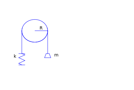
It can be shown that the vibrations of this sytem can be modeled by the following differential equation:
Home |
< Previous |
Next > |