Euler MethodsBrown University, Applied Mathematics |
MuPAD has a standard procedure to solve an initial value problem numerically. We consider two examples to demonstrate the techniques.
Example: Consider the Bernoulli equation on any interval not containing the origin subject to the initial condition:
\[ y' + y/3 = y^4 * \exp(x) , \qquad y(1) = \exp(-1/3)/3 . \]
Its solution in explicit form is known to be
\[ y(x) = (30-3*x)^{-1/3} * \exp(-x/3) , \]
so \( y(3) \approx 0.13334162798703283 \)
[f, t0, Y0] :=
[numeric::ode2vectorfield({y'(t) = (exp(t))*(y(t)^4) - (y(t)/3), y(1) = 0.23884377019126307}, [y(t)])]
or
[f, t0, Y0] := [numeric::ode2vectorfield({y'(t) = (exp(t))*(y(t)^4) - (y(t)/3), y(1) = exp(-1/3)/3}, [y(t)])]
[proc f(t,Y) ... end, 1, [exp(-1/3)/3]]
or
[numeric::ode2vectorfield({y'(t) = (exp(t))*(y(t)^4) - (y(t)/3), y(1) = exp(-1/3.0)/3.0}, [y(t)])]
[proc f(t,Y) ... end, 1, [0.2388437702]]
Then we calculate the numerical value at t=3 by typing:
[0.133341628]
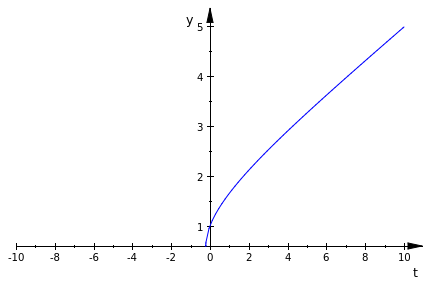
Example: Consider another example
\[ y' = 1/(3y-x-2) , \qquad y(0) =1. \]
Its solution is define dimplicitely:
\[ x=2*\exp(1-y) -5+3*y , \]
and \( y(3) \approx -0.2767313919685842 . \)
[proc Y(t) ... end
[2.52100524]
Now we plot the solution:
Euler Methods
Plotting things in MuPad is very simple. Now that you are getting more familiar with the syntax, this should be a breeze. Take the following code for instance:
Notice that there are 3 basic parameters- function, independent variable window width, and dependent window width. As with most MuPad functions, the function itself comes first. Another good parameter to use is 'GridVisible = TRUE' to turn on the grid for yourself.
To plot more than one function on the same graph, you can separate them by commas as different parameters in the same plot function.
When defining a function to plot (separate from inside the plot function), sometimes it is nice to include a parameter for the line color - 'LineColor = RGB::Red' - which literally stands for 'choose between red green and blue for your line'.
Notice that there is an extra identifier in front of the plot function this time '::Function2d'. This is just to indicate to MuPad that we want it to be a 2 dimensional graph in cases of a 3 dimensional object. In the case where you are plotting objects of multiple variables, this can be very useful. To get a 3 dimensional graph, all you have to do is change the '2' above to a '3'.
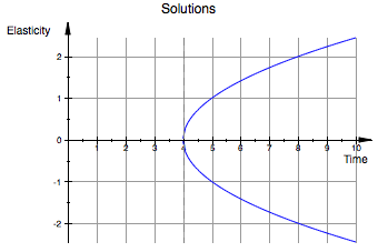
Labels are used as parameters inside the plot function. The syntax is as follows: 'Header = ['This Is My Title']' and 'AxesTitles = ['Xaxis Title', 'YAxis Title']'. Here is an example with all the aspects at once:
curve2 := (-sqrt(x -4))
plot(curve1,curve2, x=0..10, y=-5..5, Header = 'Solutions', AxesTitles = ['Time','Elasticity'],GridVisible = TRUE)
Home |
< Previous |
Next > |