Plotting Syntax in MuPADBrown University Applied Mathematics |
Plotting Syntax
MuPAD can plot many kinds of functions for you. Different kinds of plots are denoted by the extra '::' add on after the word 'plot'. The only tricky part is that sometimes you have to call 'display(%)' right after the function so that it will actually show up. Some of these kinds of plots even include animations when you click on them! To interact with plots, double click on the image and you should be able to move around, which can be very useful for 3 dimensional plots.
- Function graphs plot::Function2d, plot::Function3d
- Curves plot::Curve2d, plot::Curve3d
- Points plot::Point2d, plot::Point3d
- Lines plot::Line2d, plot::Line3d
- Polygons plot::Polygon2d, plot::Polygon3d
- Surfaces plot::Surface
- Complex objects plot::VectorField2d, plot::Ode2d, plot::Ode3d, plot::Implicit2d, plot::Implicit3d
Useful Parameters
These are things to include at the end of your plot function, seperated by commas, and stil within the parenthesis of the plot function.- GridVisible = TRUEturns on a grid for the plot
- TicksDistance = YOURNUMBERworks if the grid is visible and allows you to manipulate the size of the grid squares where YOURNUMBER is a non-negative integer
- Scaling = Constrainedforces the y-axis to have the same scale as the x-axis
- CoordinateType = LinLogforces a linear logarithmic plot
- CoordinateType = LogLogforces a logarithmic scale on both the x and y axis
- #Arrowsforces the curve to be an arrow
- #Legendcreates an automatic legend for you at the bottom of the plot
- piecewise(...)allows you to define a piecewise function to plot
Examples
Plotting Systems
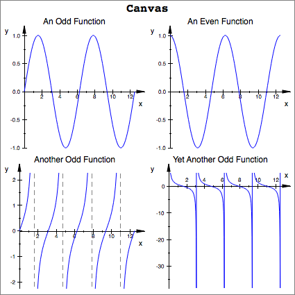
Plotting multiple functions in MuPAD is quite easy. We can use something called a canvas to accumulate several plots into a single image that you can export by right-clicking on the plot. In the following example, we will plot 4 trigonometric functions.
Header = "An Odd Function"):
Scene2 := plot::Scene2d(plot::Function2d(cos(x), x = 0..4*PI),
Header = "An Even Function"):
Scene3 := plot::Scene2d(plot::Function2d(tan(x), x = 0..4*PI),
Header = "Another Odd Function"):
Scene4 := plot::Scene2d(plot::Function2d(cot(x), x = 0..4*PI),
Header = "Yet Another Odd Function"):
Canvas := plot::Canvas(Scene1, Scene2, Scene3, Scene4,
Width = 80*unit::mm, Height = 80*unit::mm,
BorderWidth = 0.5*unit::mm,
Header = "trigonometric functions",
HeaderFont = ["Courier", Bold, 18]):
plot(Canvas)
Analytic Functions
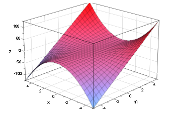
Let us take an exampleOn this function, ‘x’ is the independent variable and the range is 0 to 1. Notice the syntax. ‘plot’ command is spelled with lower case p (this is what makes Mupad plot your desired function). There is ‘asterisk (*)’ between each number and variable as this tells Mupad that you want them to be multiplied. To indicate range you let your variable, in this case ‘x’, equal to the starting number followed by two dots, then the ending number. (e.g. x= 0..77) You can put space between the staring number and the two dots and the ending number and the two dots but you cannot put a space between the two dots. (eg. x= 0 .. 77 valid, x= 0. .77 invalid, x= 0 . . 77 invalid) .
As there is more then one way to skin a cat, there indeed is more then one way to plot in Mupad. If you are a control freak and would like to control your y range you’re in luck because Mupad has a built in command plot that allows you to do so. It is the ‘plotfunc2d.’ The ‘YRange= a..b’ part allows you to control the length of the Y-axis.
plot(sqrt(x)*sin(ln(x)), x=0..1, YRange= -2..2 )

Somethings Mupad might act up and not show the plot. If this happens it means you need to show dominance; type ‘display(%)’ into your command line and this will show Mupad who’s boss.
plot::Function2d(cosh(sin(x)), x=-3..3)
display(%)
Now if you are feeling promiscuous and would like to graph multiple functions in one plot you can do so by adding a ‘,’ followed by your function.
plotfunc2d(sin(x), tan(x)/x, x^3, 3, x, x = -5..5, YRange = -100..100)
You can use the ‘plot’ command too but I like to control my Y-axis so I will use the ‘plotfunc2d’ function
Plotting Discontinuous Functions
To plot functions that aren’t defined everywhere or has a discontinuity you can just plot them using the “plot’ or ‘plotfunc2d’ function. Mupad will plot it and show dash lines where there is an asymptotes
plot(1/(x-1), x= 0..2)
To plot piecewise functions you can do so by using ’plot(piecewise( [range1, function1], [range2, function2], x = a..b)’.
plot(piecewise([0<x<2,x^2], [2<x<4, 4-x], [x>4,2]), x = 0..6)
To plot a point use ‘display(plot::Point2d( x, y)’) and to plot a list of points use ‘plot(plot::PointList2d( [[ab], [c,d]. [n,m]], Pointsize = “n”))
display(plot::Point2d(2,1))
You can add multiple function and graph them in the same plot too.
display(plot::Point2d(4,3), piecewise([0<x<2,x^2], [2<x<4, 4-x], [x>4,2]), x = 0..6, sin(x))
Implicit Plot
If you would like to plot a line or curve that satisfies an equation you can do so by using the ‘plot::Implicit2d(f(x,y), x= a..b, y = c..d))’. To plot a plane or a surface that satisfies a 3d equation use ‘plot::Implicit3d(f(x,y), x= a..b, y = c..d))’.
plot(plot::Implicit2d(3*x^2 + y^2=9, x=-2..2, y=-4..4), GridVisible = TRUE, GridLineStyle = Dotted)
Vertical and Horizontal Lines
To plot horizontal lines use ‘plot( n, x=a..b) and to plot vertical lines use ‘plot([n,none], y= a..b), where “n” is the value of the line and “a..b” is the range.
plot(2, x= -1..5)
plot([4,none], y=-3..3)
You can change the color, style, and width of the line by using ‘LineColor=RGB::”Colour”’, ‘LineStyle = “Dashed, Dotted, or Solid”’, LineWidth = “n”*unit::mm’.
plot(2, x= -1..5, LineColor = RGB::Green, LineStyle = Dashed, LineWidth = .02*unit::mm)
Now lets go to marking territories. To label your graph and your axis simplify add ‘Header = “Name”’ and ‘Axesitles = [“X-Name”, “Y-Name”]. To change tick values add ‘XTicksDistance = number, YTicksDistance = number’. To show and dictate how many ticks appear between each tick use ‘XTicksBetween = number’ (for X-asix) and ‘YTicksBetween = number’ (for Y-axis).
If you would like to show some grid you can do so by ‘GridVisible = TRUE, SubgridVisible = TRUE’. Notice this contains two commands; ‘GridVisible = TRUE’ shows the grid from the major ticks and ‘SubgridVisible = TRUE’ shows grid from the ticks in between the major ticks.
If you are fancy and would like to change the style of the grid lines you can do so by using ‘GridLineSyle’ and ‘SubgridLineStyle’ and your options are Dashed, Solid, or Dotted. You can label the curve or surface with ‘Legend = “name”’. SOMETIMES THIS DOESN’T WORK SO FIND A DIFFERENT WAY.
plotfunc2d(sin(x^2), cos(3/2), x = 0..8, Header = "LOOK", AxesTitles = ["time", "value"], XTicksDistance = .5, YTicksDistance = .2, XTicksBetween = 4, YTicksBetween = 2, GridVisible = TRUE, SubgridVisible = TRUE, GridLineStyle = Solid, SubgridLineStyle = Dashed)
plot(plot::Function2d(sin(x), x= 0..8*PI, Legend = “Sin(x)”))
Figures with Arrows
A line with an arrowhead can be drawn using ‘plot::Arrow2d([x1,y1], [x2,y2], options)’. But, sadly, Mupad does not have a builtin function that lets you draw arrowhead on a given function.Electric Circuits
We can break down an electric circuits into three parts; 1) wires and capacitors, 2) resistors, and 3) inductors. We can draw the wires, capacitors, and resistors using the ‘plot::Line2d([a,b], [c,d])’ command. Inductors will be graphed using parametric equations of a circle and using ‘plot::Curve2d([x(t), y(t)], t = a..b)’
1. Wires and Capacitors
eq1 := plot::Line2d([1,1], [3.3,1])
eq2 := plot::Line2d([3.6,1],[5,1])
eq3 := plot::Line2d([3.3,0],[3.3,2])
eq4 := plot::Line2d([3.6,0],[3.6,2])
eq5 := plot::Line2d([5,1], [5,2])
eq6 := plot::Line2d([5,3.5],[5,4])
eq7 := plot::Line2d([5,4], [4,4])
eq8 := plot::Line2d([3,4],[1,4])
eq9 := plot::Line2d([1,4],[1,2.5])
eq10 := plot::Line2d([0.5,2.5],[1.5,2.5])
eq11 := plot::Line2d([1,2],[1,1])
eq12 := plot::Line2d([0.5,2],[1.5,2],LineWidth = 1.5*unit::mm)
EQ1 := eq1, eq2,eq3,eq4,eq5,eq6,eq7,eq8,eq9,eq10,eq11, eq12
2. Resistor
eq13 := plot::Line2d([3,4],[3.1,4.5])
eq14 := plot::Line2d([3.1,4.5],[3.2,3.5])
eq15 := plot::Line2d([3.2,3.5],[3.3,4.5])
eq16 := plot::Line2d([3.3,4.5],[3.4,3.5])
eq17 := plot::Line2d([3.4,3.5],[3.5,4.5])
eq18 := plot::Line2d([3.5,4.5],[3.6,3.5])
eq19 := plot::Line2d([3.6,3.6],[3.7,4.5])
eq20 := plot::Line2d([3.7,4.5],[3.8,3.5])
eq21 := plot::Line2d([3.8,3.5],[3.9,4.5])
eq22 := plot::Line2d([3.9,4.5],[4.0,4])
EQ2 := eq13, eq14, eq15, eq16,eq17, eq18, eq19, eq20, eq21, eq22
3. Inductors
eq23 := plot::Curve2d([5 + 0.25*cos(t), 2.25 + 0.25*sin(t)], t = -PI/2..PI/2)
eq24 := plot::Curve2d([5 + 0.25*cos(t), 2.75 + 0.25*sin(t)], t = -PI/2..PI/2)
eq25 := plot::Curve2d([5 + 0.25*cos(t), 3.25 + 0.25*sin(t)], t = -PI/2..PI/2)
EQ3 := eq23, eq24, eq25
plot(EQ1, EQ2, EQ3)
Polar Plots
You can plot polar functions using the ‘plot::Polar([r,theta]), u = umin..umax,
plot::Polar([x,sin(x)], x= 0..2*PI)
Some Famous Curves
Antiversieraa := -2; b := 1; c := 1; d := 2
plot::Implicit2d(x^4 -2*a*x^3 + 4*a^2/b^2*y^2 = 0, x = -5..1, y = -2..2, Scaling = Constrained)
display(%)
plot::Implicit2d(x^4 -2*c*x^3 + 4*c^2/d^2*y^2 = 0, x = -1..5, y = -2..2, Scaling = Constrained)
display(%)
Arachnida
a:= 1; n:= 3
plot::Polar([2*a*sin(n*u)/sin((n - 1)*u),u], u= 0.0001..2*PI)
display(%)
Astroid
a:=1; b:=2; c:=3; d:=4
eq1 := plot::Implicit2d((x^2 + y^2 - a^2)^3 + 27*x^2*y^2 = 0, x= -5..5, y = -5..5)
eq2 := plot::Implicit2d((x^2 + y^2 - b^2)^3 + 27*x^2*y^2 = 0, x= -5..5, y = -5..5)
eq3 := plot::Implicit2d((x^2 + y^2 - c^2)^3 + 27*x^2*y^2 = 0, x= -5..5, y = -5..5)
eq4 := plot::Implicit2d((x^2 + y^2 - d^2)^3 + 27*x^2*y^2 = 0, x= -5..5, y = -5..5)
display(eq1, eq2, eq3, eq4)
Besace
a:= 1; b:= 1
c:= 2; d:= 2
e:= 3; f:= 3
eq1 := plot::Implicit2d((x^2 - b*y)^2 + a^2*(y^2 - x^2) = 0, x=-5..5, y=-5..5)
eq2 := plot::Implicit2d((x^2 - d*y)^2 + c^2*(y^2 - x^2) = 0, x=-5..5, y=-5..5)
eq3 := plot::Implicit2d((x^2 - f*y)^2 + e^2*(y^2 - x^2) = 0, x=-5..5, y=-5..5)
display(eq1, eq2, eq3)
Bifolium
a:=0; b:=1; c:=2; d:=3
eq0:= plot::Implicit2d((x^2 + y^2)^2 = a*x^2*y, x= -1..1, y= -0.2..1)
eq1:= plot::Implicit2d((x^2 + y^2)^2 = b*x^2*y, x= -1..1, y= -0.2..1)
eq2:= plot::Implicit2d((x^2 + y^2)^2 = c*x^2*y, x= -1..1, y= -0.2..1)
eq3:= plot::Implicit2d((x^2 + y^2)^2 = d*x^2*y, x= -1..1, y= -0.2..1)
display(eq0, eq1,eq2,eq3)
Cardioid
plot(plot::Polar([(1-cos(u)),u], u=0..2*PI), plot::Polar([2*(1-cos(u)),u], u =0..2*PI), plot::Polar([3*(1-cos(u)),u], u = 0..2*PI))
Cramer
plot(plot::Implicit2d(x*(x^2 + y^2) = 3*x^2 - y^2, x = -1..5, y = -5..5))
Cycloid
WheelRadius := 1:
WheelCenter := [x, WheelRadius]:
WheelRim := plot::Circle2d(WheelRadius, WheelCenter,
x = 0..4*PI,
LineColor = RGB::Black):
WheelHub := plot::Point2d(WheelCenter, x = 0..4*PI,
PointColor = RGB::Black):
WheelSpoke := plot::Line2d(WheelCenter,
[WheelCenter[1] + 1.5*WheelRadius*sin(x),
WheelCenter[2] + 1.5*WheelRadius*cos(x)],
x = 0..4*PI, LineColor = RGB::Black):
color:= [RGB::Red, RGB::Green, RGB::Blue]:
r := [1.5*WheelRadius, 1.0*WheelRadius, 0.5*WheelRadius]:
for i from 1 to 3 do
Point[i] := plot::Point2d([WheelCenter[1] + r[i]*sin(x),
WheelCenter[2] + r[i]*cos(x)],
x = 0..4*PI,
PointColor = color[i],
PointSize = 2.0*unit::mm):
Cycloid[i] := plot::Curve2d([y + r[i]*sin(y),
WheelRadius + r[i]*cos(y)],
y = 0..x, x = 0..4*PI,
LineColor = color[i]):
end_for:
plot(WheelRim, WheelHub, WheelSpoke,
Point[i] $ i = 1..3,
Cycloid[i] $ i = 1..3,
Scaling = Constrained,
Width = 120*unit::mm, Height = 60*unit::mm):
Galileo’s Spiral
plot(plot::Polar([-r^2 - 10,r], r = 0..6*PI))
Kiepert
a:= 1; b:=2; c:=3
eq1:=plot::Polar([(a^3*cos(3*u))^(1/3),u], u= -2*PI..2*PI)
eq2:=plot::Polar([(b^3*cos(3*u))^(1/3),u], u= -2*PI..2*PI)
eq3:=plot::Polar([(c^3*cos(3*u))^(1/3),u], u= -2*PI..2*PI)
plot(eq1,eq2,eq3)
Limacon
plot(plot::Polar([1.5+3*cos(x), x], x = 0..2*PI))
Rose
plot(plot::Polar([cos(3*u),u], u= 0..PI))
Trefoil
plot(plot::Curve2d([(2*cos(2*t) - cos(t)), (2*sin(2*t) + sin(t))], t=0..10))
Home |
< Previous |
Next > |