II. Plotting functions

---

Plotting in Maple is simple, but there is much to plotting than one may think. Let’s begin by looking at the basic syntax of the plot command in Maple:

>plot(function, range, options(if any));

As you can see, the plot function involve a function, the x and y ranges of the plot, and any conditions if there are any present. The x and y ranges do not necessarily have to be inputted, but if there are other functions to plot (mentioned later), it is best to make the plot fit all functions by inputting the appropriate ranges. If you do not input a range for one function, then Maple will automatically generate a plot that fits the function. There are many options to choose from when using all types of plot commands. The most important options that can be used for ODEs are listed below, but others are listed in the Maple website

Option	Code Input	Notes
Specify type of axes	axes=f	The value f can be boxed, framed, none, or normal. This option is automatically set to normal if not specified.
Coordinate system used for displaying axes	axiscoordinates=t	The value t can be either polar or Cartesian. This option is automatically set to Cartesian if not specified.
Specifying color for curves to be plotted	color=n OR colour=n	The value n can be replaced with any color. For simplicities sake, it’s best to use simple colors such as blue and red. This option is automatically set to the default color of the plot command (which is usually red).
Detecting discontinuities	discont=t	If a discontinuity exists in the specified function for plotting, then the t value is true. This option is automatically set to false if not specified.
Labeling axes	labels=[x,y]	This option specifies what the axes in the plot is labeled with. By default they have no labels.
Legend entry	legend=s	This option can be used for displaying a legend entry for each curve in the plot. The s value can be whatever the user desires. This option is automatically nonexistent if not specified.
Scaling of the graph	scaling=s	The s value can be constrained or unconstrained. The default value is unconstrained, which means the plot is scaled to fit the window. The constrained value makes all axes use the same scale so, for example, a circle would appear perfectly round.
Symbols used to plot graph	symbol=s	The s value can be asterisk, box, circle, diagonalcross, diamond, point, solidcircle, soliddiamond, or solidbox. This option is automatically nonexistent if not specified.
Title of graph	title=t	This option can be used for displaying a title for the plot. This option is automatically nonexistent if not specified.

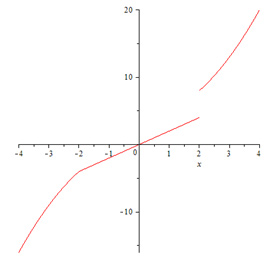
Let’s plot a piecewise function:

> f:= piecewise(x<=-2,-x^2,-2<=2, 2*x,x>2,x^2+4);
> plot(f(x), x=-4..4, discont=true);

This should generate the following plot:

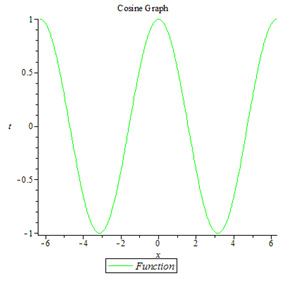
Let’s make a plot using as many of the options as possible:

> (cos(x),x=-2*Pi..2*Pi,title=”Cosine Graph”, axes=framed, axiscoordinates=Cartesian,color=green,labels=[x,t],legend=Function);

This input generates the below graph:

III. Plotting with axes, without axes

---

There are times when the axes could interfere with displaying certain functions and solutions to ODEs. Fortunately, getting rid of axes in recent versions of Maple is very easy.
One method of specifying axes is to use the above options, but there is also a visual method of changing axes.

Simply right-click the graph that is generated by Maple, and go to the tab labeled “Axes,” and click on “None” to remove the axes from the graph. If you wish to make them appear, make sure the “None” is unchecked. You may also see the axes boxed or framed.

*Note that some options, such as style, point, line, axes, and color, can be altered by right-clicking the graph and changing the details accordingly.

IV. Implicitplot command

---

*Refer to Maple file “Defining Functions”

There are many plot commands in Maple, and the implicitplot command is very useful for plotting implicitly defined functions (which is very useful for visualizing an ODE problem).
Let’s look at the basic of the syntax of the implicitplot command:

> implicitplot(function, x and y ranges, options);

The implicitplot can be used to plot functions such as circles, functions that involves multiple variables, polar equations, etc. Note that the plots package has to opened.
Let’s plot a circle:

> with(plots):
> implicitplot(x^2+y^2=4,x=-3..3,y=-3..3);

Now let’s try plotting a polar equation:

> implicitplot(r=1-cos(theta), r=0..2, theta=0..2*Pi, coords=polar);

This generates the following plots:

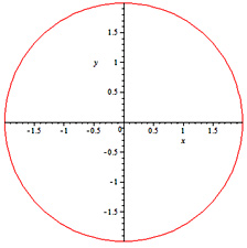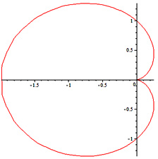Circular Plot	Polar Plot

As you can see, you can practically plot any implicit function using the implicitplot command. Explicit functions can be plotted using the regular plot command.

V. Displaying multiple plots in the same/separate

---

*Refer to Maple file “Defining Functions”

Drawing multiple plots is easy, and displaying them on the same or separate plan just adds another step. In order to display them on the same plane, use the display command. The syntax is as follows (for three functions):

> display({function1, function2, function3}, options);

The functions, to prevent human error, can be expressed by variables by defining them. The options listed above can be used for this command as well. Note that the plots package has to be opened as well.

For example:

> with(plots):
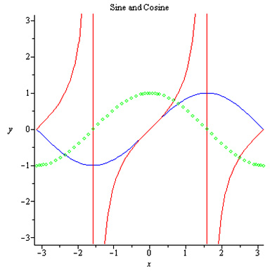
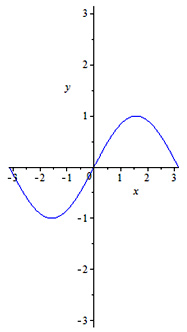
> F:=plot(sin(x),x=-Pi..Pi.y=-Pi..Pi,color=blue):
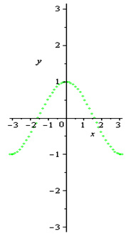
> G:=plot(cos(x),x=-Pi..Pi,y=-Pi..Pi,style=point,color=green):
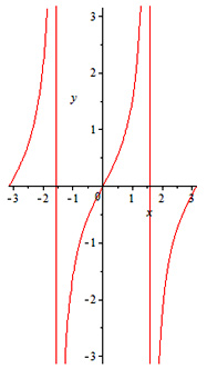
> H:=plot(tan(x),x=-Pi..Pi,y=-Pi..Pi,style=line):
> display({F,G,H},axes=framed,scaling=constrained,title=”Sine and Cosine”);

This generates the following graph:

Displaying multiple plots separately can be done in one of two ways. You may either plot each function independently, or you may use the Array command. Using the F, G, and H plots above, we can display the plots separately:

> A:=Array(1..3):
> A[1]:= F:
> A[2]:= G:
> A[3]:= H:
> display(A);

Note that the options of the graphs F, G, and H are carried over from the implicitplot command. If you wish to revert the options of each plot, it’s best to enter the restart command and fix the options where the plots F, G, and H are defined.

*Note: If you wish to copy the output of Maple to enter into a word processor, make sure to change the font of the output to monospaced, because the default output of Maple is an image and not text.

For implicit plotting, a similar syntax can be used:

c implicitplot([x^2-y^2=2,y=exp(x)+2],x=-Pi..Pi,y=-Pi..Pi,color=[red,black],legend=[function1,function2]);

This generates the following plot:

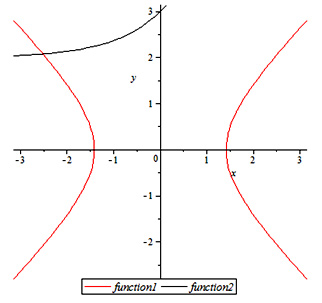
As you can see in the input, there are a couple of things to note:

1. Exponential functions, which is normally expressed as e^x, is inputted as “exp().”
2. When displaying multiple functions (this applies to the normal plot command as well), you must combine them using brackets []. Any subsequent options are applied in the order respective to the initial input. In this example, the first function x²-y²=2 is red and is labeled function1 because the color and legend options specify those options in the brackets.

 

VI. Reverse Axes

---

How to reverse the axes, we show on example.

restart;
with( plots ):
p0 := plot( x^2, x=0..1 ):

The plottools package provides a transform command that creates a transformation that can be applied to a plot data structure.

REV := plottools:-transform( (x,y)->[1-x,1-y] ):
display( REV(p0) );

Now, to reverse the labels on the axes, use the enhanced tickmarks optional argument to plot:

display( REV(p0), tickmarks=[[1=0,0.5=1/2,0=1],[1=0,0.5=1/2,0=1]] );

We modify REV so that it plots in the third quadrant:

REV2 := plottools:-transform( (x,y)->[-x,-y] ):
display( REV2(p0), tickmarks=[[0=0,-0.5=1/2,-1=1],[0=0,-0.5=1/2,-1=1]] );
EV2 := plottools:-transform( (x,y)->[-x,-y] ):
display( REV2(p0), tickmarks=[[0=0,-0.5=1/2,-1=1],[0=0,-0.5=1/2,-1=1]] );

 

2. Solving ODEs: dfieldplot, DEplot, odeplot, Defining Function as Solution, Nullclines

I. Solving Using Direction/Slope Fields (dfieldplot)

---

*Refer to Maple file “Direction Fields”

When solving ODEs, there are many methods in plotting them. In this section, we will learn how to use three plot commands in the DEtools package to plot the solutions to ODEs. The dfieldplot command draws out a direction/slope field of the given function. The generic syntax of the command is as follows:

> with(DEtools):
> dfieldplot(differential equation, independent variable, x range, y range);

In order to express a differential equation, for example a function of y in relation to x, you must enter “diff(y(x),x).” This can be also expressed as “D(y)(x),” but for simplicities sake, we will use the former expression.
Try out the following:

> dfieldplot(diff(y(x),x)=y(x)*(1-y(x)), y(x), x=-2..2, y=-2..2);

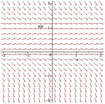
The input should generate the above direction field. Unfortunately, you must plot differential equations using dfieldplot explicitly. Therefore, it is best to solve a given differential equation to express it explicitly if it is given implicitly.

II. Solving Using DEplot

---

*Refer to Maple file “Direction Fields”

If you wish to plot the solutions to the differential equations in a slope field, you must use the DE plot command. The parameters to enter are the same as the dfieldplot command, but includes the initial values and any options.Therefore, the generic syntax of the DEplot command would be:

> DEplot(differential equation, independent variable, x range, y range, Initial Value(s), Line Color);

Try the following example which involves Newton’s law of cooling:

> ode:=diff(y(t),t)=k*(Am-y(t)): Am:=20: k:=0.1:
> ivs := [y(0)=20, y(0)=30, y(0)=50]:
> DEplot(ode,y(t),t=0..50,y=0..100,ivs,linecolor=blue);

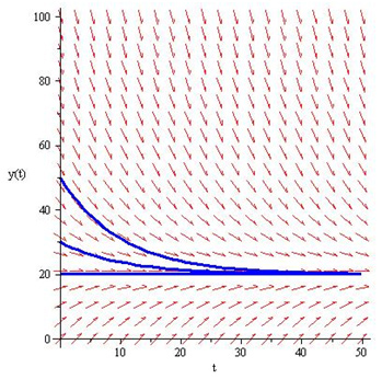
The input should generate the above direction/slope field with three curves approaching y(t)=20. Note that the initial values used for the DEplot command can be in the form of an array using brackets. Unfortunately, for DEplot, like dfieldplot, the differential equations must be expressed explicitly.

III. Solving Using odeplot

---

*Refer to Maple file “Direction Fields”

The odeplot command is slightly different than the DEplot, and is slightly enhanced compared to the dfieldplot. Compared to other plot commands, odeplot has the ability to animate the solution to an ODE. Note that the odeplot command is within the plot package, not the DEtools package. The generic syntax of the odeplot command is fairly easy and is as follows:

> odeplot(dsolve({differential equation, initial value}, type=numeric, range)

The dsolve command solves the differential equation. Plotting the result will give us a graph of the solution to the ODE. The type=numeric option finds a numerical solution for the differential equation.
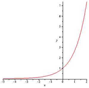
Let’s see this in a simple example:

> with(plots) :
> ode :=dsolve({diff(y(x),x)=y(x),y(0)=1},type=numeric, range=-5..2) :
> odeplot(ode);

This should generate the following graph:

IV. Plotting Vertical Lines

---

*Refer to Maple file “Vertical Line”

Plotting vertical lines is fairly straightforward and easy. Since vertical lines are expressed with constants in terms of x, simply use the implicitplot command and input the equations. For example, let’s draw one horizontal line at y=1 and one vertical line at x=Pi/2:

> with(plots):
> a:=implicitplot(y=1,x=-3..3,y=-2..2);
> b:=implicitplot(x=Pi/2,x=-3.33,y=-1..2, color=yellow, linestyle=3,thickness=2);
> display(a,b);

This should result in the following graph:

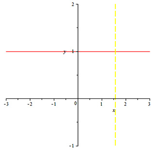
Note that the linestyle option changes the type of line drawn, and the thickness adjusts the thickness of the specific line. For the linestyle option, 1=solid line, 2=dots, 3=dashes, 4= dashes and dots, 5= bold dashes, etc.

 

 

 

 

 

 

 

 

 

 

 

 

5. Numerical Solutions: Plotting Difference Between Exact and Approximate in Regular Plot/Log Plot

---

Explanation of syntax:

Some parts of the syntax of the code may be confusing, so that will be explained here. You may wonder why the variable x[k] and y[k] are used instead of x(k) and y(k). The reason is because the brackets [] resemble the denotation you see. Therefore, x[k] and y[k] in actual form would be xk and yk respectively. The parenthesis, on the other hand, would resemble the independent variable relevant to the dependent variable in the parenthesis.

The variable k1 denotes the equation f(x,y) which is subject to differentiation in subsequent orders of the Taylor expansion. The variables k2 is the differentiation of k1, and k3 is the differentiation of k2, and so forth.

The lines with “for [variable] from [initial value] to [final value] do” and “end do” is a loop. A loop in programming terms is basically a recursion in which any computation that is entered between these lines. The loop begins with the “for [variable] from [initial value] to [final value] do” and ends with the “end do” or “od.” The variable can be any value so long as the recursion uses that same variable (If you use k, make sure to use k as the reference variable for entering k-1, k+1, etc.). The initial value is the sequential number that the recursion should begin with, which in this case should be 1. The final value is the last sequential number that the recursion should end with, which in this case should be 10, since 10 increments is enough for a valid numerical approximation. The “end do” must be there for the loop to end. If you do not put this, Maple will give you an error. To avoid Maple from providing you with a long output, make sure to end all lines with colons “:” instead of semi-colons “;”. This will suppress the output into a smaller output.

I. Euler’s Method

---

*Refer to the Maple file “Euler’s Method”

*Euler method commands are available in Maple, but this is to demonstrate how differential equations will be calculated manually, which will also allow for plotting.
Using the Euler command only requires one line of code, but this section will show what calculations are conducted within that one line of code.

> with(Student[NumericalAnalysis]):
> Euler(diff(z(t),t)=1/(2*t-3*z(t)+5),z(0)=1,t=1,output=plot);

The Euler’s method takes the current y term and adds it with the difference of the current and next x term multiplied by the function in terms of the current x and y terms to yield the next y term.
Therefore, the generic Maple syntax will be as follows:

> f:= some equation
> x[0]:= some value
> y[0]:= some value
> h:= some value # represents the difference between the x terms, x[k+1]-x[k]
> for k from 0 to 9 do
> x[k+1]:=x[k]+h:
> y[k+1]:=y[k]+h*f(x[k],y[k]):
> end do

Let’s apply this syntax to an example where we have a differential equation of y’=1/(2x-3y+5) and the initial conditions are y(0)=1 and h=0.1 (This equation and initial conditions will be used in subsequent examples):

> f:= (x,y)->1/(2*x-3*y+5);
> x[0]:=0:
> y[0]:=1:
> h:=0.1:
> for k from 1 to 10 do
> x[k]:=k*h:
> y[k]:=y[k-1]+h*f(x[k-1],y[k-1]):
> end do

II. Backwards Euler’s method

---

*Refer to the Maple file “Backward Euler’s Method”

The Backward Euler’s method is another method of approximation. The syntax of the Backwards Euler Method is much like the Euler Method but instead of multiplying the value step size (h) by the value of function in the current term, it is multiplied by the value of the function of the next term.
Therefore, the Maple syntax will be as follows:

> f:= (x,y)->1/(2*x-3*y+5);
> x[0]:= 0:
> y[0]:= 1:
> h:= 0.1:
> for k from 0 to 9 do
> x[k+1]:= x[k]+h:
> bb := solve(b=y[k]+h*f(x[k+1],b),b);
> y[k+1]:= evalf(min(bb));
> end do;

The minimum is determined here because this is a quadratic equation which has 2 roots and thus we much choose the smaller root.

III. Trapezoid Rule

---

*Refer to the Maple file “Trapezoid Rule”

The concept of the Trapezoidal Rule in numerical methods is similar to the trapezoidal rule of Riemann sums. The Trapezoid Rule is generally more accurate than the above approximations, and it calculates approximations by taking the sum of the function of the current and next term and multiplying it by half the value of h.
Therefore the Maple syntax will be as follows:

> f:= (x,y)->1/(2*x-3*y+5);
> x[0]:= 0:
> y[0]:= 1:
> h:= 0.1:
> for k from 0 to 9 do
> x[k+1]:= x[k]+h:
> bb := solve(b=y[k]+(h/2)*(f(x[k],y[n])+f(x[n+1],b)),b);
> y[k+1]:= evalf(min(bb));
> end do;

IV. Improved Euler’s method

---

*Refer to the Maple file “Improved Euler’s Method”

The Improved Euler’s method, also known as the Heun formula or the average slope method, gives a more accurate approximation than the trapezoid rule and gives an explicit formula for computing y(n+1) in terms of the values of x. The syntax of the Improved Euler’s method is similar to that of the trapezoid rule, but the y value of the function in terms of y(n+1) consists of the sum of the y value and the product of h and the function in terms of x(n) and y(n).
Therefore, the Maple syntax will be as follows:

> f:= (x,y)->1/(2*x-3*y+5);
> x[0]:=0:
> y[0]:=1:
> h:=0.1:
> for n from 1 to 10 do
> x[n]:=x[n]*h:
> ystar:=y[n-1]+h*f(x[n-1],y[n-1]):
> y[n]:=y[n-1]+(h/2)*(f(x[n-1],y[n-1])+f(x[n],ystar):
> od;

V. Modified Euler’s method

---

*Refer to the Maple file “Modified Euler’s Method”

The Modified Ruler’s method is also called the midpoint approximation. This method reevaluates the slope throughout the approximation. Instead of taking approximations with slopes provided in the function, this method attempts to calculate more accurate approximations by calculating slopes halfway through the line segment. The syntax of the Modified Euler’s method involves the sum of the current y term and the product of h with the function in terms of the sum of the current x and half of h (which defines the x value) and the sum of the current y and the product of the h value and the function in terms of the current x and y values (which defines the y value).
Therefore, the Maple syntax is as follows:

f:= (x,y)->1/(2*x-3*y+5);
> x[0]:=0:
> y[0]:=1:
> h:=0.1:
> for k from 1 to 10 do
> x[k]:=k*h:
> y[k]:=y[k-1]+h*f(x[k-1]+(h/2),y[k-1]+(h/2)*f(x[k-1],y[k-1])):
> end do

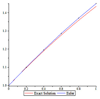
Let’s take all of the approximations and the exact values to compare the accuracy of the approximation methods: *Refer to the Maple file “Exact Values” for the exact values.

x values	Exact	Euler	Backwards Euler	Trapezoid	Improved Euler	Modified Euler
0.1	1.049370088	1.050000000	1.057930422	1.0493676	1.049390244	1.049382716
0.2	1.097463112	1.098780488	1.118582822	1.0974587	1.097594738	1.097488615
0.3	1.144258727	1.146316720	1.182399701	1.1442530	1.144322927	1.144297185
0.4	1.189743990	1.192590526	1.249960866	1.1897374	1.189831648	1.189795330
0.5	1.233913263	1.237590400	1.322052861	1.2339064	1.234025039	1.233977276
0.6	1.276767932	1.281311430	1.399792164	1.2767613	1.276904264	1.276844291
0.7	1.318315972	1.323755068	1.484864962	1.3183102	1.318477088	1.318404257
0.8	1.358571394	1.364928769	1.580059507	1.3585670	1.358757326	1.358671110
0.9	1.397553600	1.404845524	1.690720431	1.3975511	1.397764204	1.397664201
1.0	1.435286691	1.443523310	1.830688225	1.4352865	1.435521666	1.435407596
Accuracy	N/A	99.4261%	72.4513%	99.9999%	99.9836%	99.9916%

Notice how each improved approximation approaches the exact value, which results in the modified Euler’s method being the most accurate method of approximating the value of the differential equation y’=1/(2*x-3*y+5). Note that the modified Euler’s method isn’t always the most accurate approximation method, as the improved Euler’s method can be more accurate than the modified Euler’s method depending on the differential equation in question.

Polynomial Approximation using Taylor series expansions

---

*The examples used for this section is related to the Cauchy example in the Analytical Solutions chapter.

VI. First Order Polynomial Approximation

---

*Refer to Maple file “First Order Polynomial Approximation”

Approximations using Taylor series expansions is a much easier task to perform using Maple because there are many iterations of the same calculations performed in order to achieve the desired answer.

Approximations with using Taylor series expansions in the first-order is actually the Euler algorithm: y_n+1=y_n+hf(x_n,y_n)=y_n+h/(1-2x_n+y_n), n=0,1,2,…

> f:= (x,y)->1/(2*x-3*y+5);
> x[0]:=0:
> y[0]:=1:
> h:=0.1:
> for k from 0 to 9 do
> x[k+1]:=x[k]+h:
> y[k+1]:=y[k]+h*f(x[k],y[k]):
> end do

They are similar in that they both take in the current term and add the approximate deviation to the next term in order to yield the value of the next term. If you look at the Maple file, the approximation of the sequence is the last y term of the sequence, which in this case is y₁₀=1.443523310.

For each step in the sequence, the expansion requires 3 addition, 1 subtraction, 3 multiplication, and 1 division operations. Since there are 8 steps to this sequence, in order to obtain the desired approximation, the code performs 80 operations, which would be hectic work to do by hand.

VII. Second Order Polynomial Approximation

---

*Refer to Maple file “Second Order Polynomial Approximation”

The second order Taylor approximation is just adding the second order differential deviation to the next term in the same equation used for the first order Taylor expansion. The approximation is y10=1.435290196. This algorithm requires 22 operations per step, which means that the entire sequence requires 220 steps. However, this is not significant since Maple does all the work.

Here is the syntax for the second order Taylor approximation:

> f:= (x,y)->1/(2*x-3*y+5);
> x[0]:=0:
> y[0]:=1:
> h:=0.1:
> for k from 0 to 9 do
> x[k+1]:=x[k]+h:
> k1:=f(x[k],y[k]):
> k2:=-(4*x[k]-6*y[k]+7)/2*x[k]-3*y[k]+5)^3:
> y[k+1]:=y[k]+h*k1+k2*h^2/2:
> end do:
> taylorapproximation2:=seq([x[k],y[k]],k=0..10);

*Notice that the taylorapproximation2 yields only the final values of x and y as opposed to showing all values determined for each equation within the recursion.

The above syntax is correct if the y” of the original differential equation (represented by k2) is solved by hand. However, there is a way to work around this to lessen handwork and let Maple do a majority of the work.

*Refer to Maple file “Second Order Polynomial Approximation Other Method”

Inside the loop, all you have to do is rewrite k2 and insert additional code to let Maple solve the derivative of the differential equation in terms of x and y.
Below would be the revised loop for the second order Taylor approximation:

> for k from 0 to 9 do
> x[k+1]:=x[k]+h:
> k1:=f(x[k],y[k]):
> fx:=subs(t=x[k],u=y[k],diff(f(t,u),t)) :
> fy:=subs(t=x[k],u=y[k],diff(f(t,u),u)) :
> k2:=(fx+fy*k1):
> y[k+1]:=y[k]+h*k1+k2*h^2/2:
> end do:
> taylorapproximation2:=seq([x[k],y[k]],k=0..10);

VIII. Third Order Polynomial Approximation

---

*Refer to Maple file “Third Order Polynomial Approximation”

The third order Taylor approximation is adding a third order differential deviation to the equation for the 2nd order expansion. The approximation for this is y₁₀=1.435283295.
Here is the syntax for the third order Taylor approximation:

> f:= (x,y)->1/(2*x-3*y+5);
> x[0]:=1:
> y[0]:=2:
> h:=0.1:
> for k from 0 to 9 do
> x[k+1]:=x[k]+h:
> k1:=f(x[k],y[k]):
> fx:=subs(t=x[k],u=y[k],diff(f(t,u),t)) :
> fy:=subs(t=x[k],u=y[k],diff(f(t,u),u)) :
> k2:=(fx+fy*k1):
> fxx:=subs(t=x[k],u=[k],diff(f(t,u),t,t)):
> fxy:=subs(t=x[k],u=[k],diff(f(t,u),t,u)):
> fyy:=subs(t=x[k],u=[k],diff(f(t,u),u,u)):
> k3:= (fxx+2*fxy*k1+fyy*k1^2+fx*fy+fy^2*k1):
> y[k+1]:=y[k]+h*k1+k2*h^2/2+h^3/6*k3:
> end do:
> thirdtaylorapproximation:=seq([x[k],y[k]],k=0..10);

The total number of numerical operations here is 420. It is obvious at this point why using mathematical programs such as Maple is a desired approach for such problems.

XI. Regular Plotting vs. Log-Plotting

---

*The example for this section is related to the Cauchy example in the Analytical Solutions chapter and Taylor Approximations section of this chapter.”

*Refer to the Maple file “Plotting and log plotting.”

Plotting the absolute value of the errors for Taylor approximations, such as the ones from the previous example, is fairly easy to do in normal plotting.

The normal plotting procedure involves taking all of the information in the three Maple files regarding the Taylor approximations and putting them into one file, then calculate the exact solution, then find the difference between each approximation and the exact solution, and plotting the solution.

Looking at the code, the syntax is pretty much self-explanatory. The only part that may confuse students is the syntax for the plot command. The plot command need not be in the same syntax as the file has it. If you wish to, you can alter the syntax to form a curve instead of dots.

Log-plotting is not much different than plotting normally. In other programs such as Mathematica, there are a couple of fixes to make, but in Maple only one line of code is required, as seen in the file. Make sure that before you use the logplot command to open the plots package.

X. Runge-Kutta Method

---

*Refer to the Maple file “Runge-Kutta Method.”

The most common order of Runge-Kutta method used is the fourth order, in which four iterations of calculations are used to make an approximation. The first and second orders do exist, but the Euler methods actually are Runge-Kutta methods. The standard Euler’s method is the first order Runge-Kutta method, and the Improved Euler’s Method is the second order Runge-Kutta method.

The fourth order Runge-Kutta method is a slightly different method of approximation, since it incorporates more levels of iterations to narrow down approximations. For this method, we will use the same non-linear differential equation we have used for the Euler methods and Polynomial approximations.

The syntax for this method is as follows:

> f:= (x,y)->1/(2*x-3*y+5);
> x[0]:=0:
> y[0]:=1:
> h:=0.1:
> for n from 1 to 10 do
> x[n]:=n*h:
> k1:=f(x[n-1],y[n-1]):
> k2:=f(x[n-1]+(h/2),y[n-1]+(h/2)*k1):
> k3:=f(x[n-1]+(h/2),y[n-1]+(h/2)*k2):
> k4:=f(x[n-1]+h,y[n-1]+h*k3):
> y[n]:=y[n-1]+(1/6)*(k1+2*k2+2*k3+k4):
> od;

Now, let’s compare the exact value and the values determined by the polynomial approximations and the Runge-Kutta method.

x values	Exact	First Order Polynomial	Second Order Polynomial	Third Order Polynomial	Runge-Kutta Method
0.1	1.049370088	1.050000000	1.049375000	1.049369792	1.049370096
0.2	1.097463112	1.098780488	1.097472078	1.097462488	1.097463129
0.3	1.144258727	1.146316720	1.144270767	1.144257750	1.144258752
0.4	1.189743990	1.192590526	1.189758039	1.189742647	1.189744023
0.5	1.233913263	1.237590400	1.233928208	1.233911548	1.233913304
0.6	1.276767932	1.281311430	1.276782652	1.276765849	1.276767980
0.7	1.318315972	1.323755068	1.318329371	1.318313532	1.318316028
0.8	1.358571394	1.364928769	1.358582430	1.358568614	1.358571457
0.9	1.397553600	1.404845524	1.397561307	1.397550500	1.397553670
1.0	1.435286691	1.443523310	1.435290196	1.435283295	1.435286767
Accuracy	N/A	99.4261%	99.99975%	99.99976%	99.99999%

You will notice that compared to the Euler methods, these methods of approximation are much more accurate because they contains much more iterations of calculations than the Euler methods, which increases the accuracy of the resulting y-value for each of the above methods.

6. Laplace Transforms

---

Laplace transforms and Inverse Laplace Transforms

Laplace transforms in Maple is really straightforward and doesn’t require any complicated loops like the numerical methods.

For example, let’s take the equation t^2+sin(t)=y(t) as our equation. The syntax for finding the laplace transform of this equation requires the simple syntax below:

> with(inttrans):
> laplace (t^2+sin(t)=y(t),t,s) ;

Yes, that is all. Easy, right? The syntax for the command is (equation, dependent value, independent value).

Finding the inverse Laplace transform requires a similar syntax. Just take the result we have from the Laplace transform above and apply it here:

> with(inttrans):
> invlaplace ((2/s^3)+(1/s^2+1),s,t);

Very easy indeed. The syntax for the inverse Laplace transform is reversed compared to the Laplace transform for some reason. The syntax is (equation, independent value, dependent value).

Solving equations with periodic piecewise continuous functions

> with(plots):
> with(inttrans):
> E:=1; a:=2;
> yh :=t->invlaplace((x+5+2)/(x^2+5*x+6), x, t);
> p := x^2+5*x+6;
> yp1 := t->invlaplace(E/(a*x^2*(x^2+5x+6)),x,t)
> yp2 := t->invlaplace(E*exp(-a*x)/(x*p*(1-exp(-a*x))), x, t)
> y := t-> yp1(t)-piecewise(a < t, yp2(t-a), 2*a < t, yp2(t-2*a), 3*a < t, yp2(t-3*a))
> plot(y(t), t = 0 .. 4*a);
> y2 := t->y(t)+yh(t)
> plot(y2(t), t = 0 .. 4*a);