We use polar coordinates as an alternative way to describe points
in the plane. In polar coordinates, we describe points via their angle
(called argument or polar angle) with
the positive x-axis measured in counterclockwise direction, and the
distance from the origin (called radial distance). See figure below.
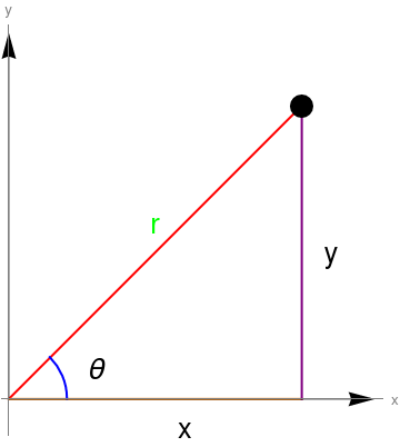
From this picture, it should be clear that we can switch back and forth between the Cartesian coordinate system and polar coordinate system in the following manner:
\[
x= r\,\cos \theta , \qquad y = r\,\sin \theta ,
\]
and
\[
r = \sqrt{x^2 + y^2} \ge 0, \qquad \theta = \begin{cases} \arctan \left( \frac{y}{x} \right) , & \ \mbox{ if } \ x > 0 , \\
\arctan \left( \frac{y}{x} \right) + \pi , & \ \mbox{ if } \ x < 0
\mbox{ and } \ y\ge 0, \\
\arctan \left( \frac{y}{x} \right) - \pi , & \ \mbox{ if } \ x < 0
\mbox{ and } \ y< 0, \\
\frac{\pi}{2} , & \ \mbox{ if } \ x=0 \mbox{ and } \ y> 0, \\
-\frac{\pi}{2} , & \ \mbox{ if } \ x=0 \mbox{ and } \ y< 0, \\
\mbox{undefined} & \ \mbox{ if } \ x=0 \mbox{ and } \ y =0 .
\end{cases}
\]
Note the argument is a multivalued function and above formula is used to
define its principle value.
Here are some examples of polar plot.