Prof. Vladimir A. Dobrushkin
This tutorial contains many matlab scripts.
You, as the user, are free to use all codes for your needs, and have the right to distribute this tutorial and refer to this tutorial as long as this tutorial is accredited appropriately. Any comments and/or contributions for this tutorial are welcome; you can send your remarks to
RC circuits
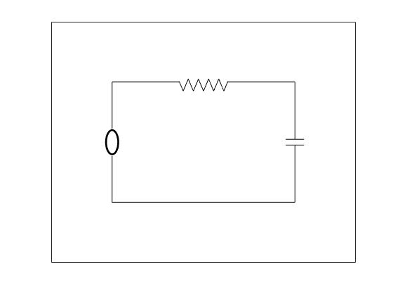
Suppose that we wish to analyze how an electric current flows through a circuit. An RC circuit is a very simple circuit might contain a voltage source, a capacitor, and a resistor (see Figure). A battery or generator is an example of a voltage source. The glowing red heating element in a toaster or an electric stove is an example of something that provides resistance in a circuit. A capacitor stores an electrical charge and can be made by separating two metal plates with an insulating material. Capacitors are used to power the electronic flashes for cameras. Current, I(t), is the rate at which a charge flows through this circuit and is measured in amperes or amps (A). We assign a direction to the current. A current flowing in the opposite direction will be given negative values.
% Wires and Window
plot([-3;3],[-1;-1],'black')
hold
plot([1;3],[1;1],'black')
xlim([-5 5])
ylim([-2 2])
set(gca,'xtick',[])
set(gca,'ytick',[])
%Resistor
plot([-3;-0.8],[1;1],'black')
plot([0.8;1],[1;1],'black')
t = -0.8:1/1000:0.8;
r = 0.1*sawtooth(2*pi*3*t,0.5)+0.95;
plot(t,r,'black')

%Capacitor
plot([3;3],[1;0.05],'black')
plot([3;3],[-.05;-1],'black')
plot([2.7;3.3],[.05;.05],'black')
plot([2.7;3.3],[-.05;-.05],'black')

% circle
plot([-3;-3],[1;0.2],'black')
plot([-3;-3],[-0.2;-1],'black')
viscircles([-3 0],0.2,'Color','black')
The source voltage, E(t), is measured in volts (V). Kirchhoff's Second Law tells us that the impressed voltage in a closed circuit is equal to the sum of the voltage drops in the rest of the circuit. Thus, we need only compute the voltage drop across the resistor, ER, and the voltage drop across the capacitor, EC. According to Kirchhoff's Law, this is
We will now investigate how our circuit reacts under different voltage sources. For example, we might have a zero voltage source (the capacitor could still hold a charge). We could also have a constant nonzero source of voltage such as a battery or a fluctuating source of voltage such as a generator. We might even have a series of pulses of voltage where the current is periodically turned on and off. We would like to be able to understand the solutions to the above differential equation for different voltage sources E(t). If we view the differential equation as an expression for computing how fast current is flowing across the capacitor, we can analyze our circuit from a geometric point of view and can actually say a great deal about circuits without solving a differential equation.
Example: We consider a simplest case when there is no voltage source in the circuit. In this case, the equation
Example: If we assume that we have a nonzero constant source of voltage, E(t) = K, in our circuit such as a battery, then we obtain the separable differential equation
Example: If we attach a battery to our circuit at time t=0 and then disconnect the battery at t=5, then we obtain a piecwise continuous voltage function. For example, if
st5 = StreamPlot[{1, -y}, {t, 5, 12}, {y, -3, 12}, PlotRange -> {{Full, {5, 12}}, Full}]
Show[st, st5]

s1 = NDSolve[{y'[t] + y[t] == EC[t], y[0] == 1}, y, {t, 0, 30}]
p1 = Plot[Evaluate[y[t] /. s1], {t, 0, 20}, PlotStyle -> {Thick, Red}]
s2 = NDSolve[{y'[t] + y[t] == EC[t], y[0] == -2}, y, {t, 0, 30}]
p2 = Plot[Evaluate[y[t] /. s2], {t, 0, 20}, PlotStyle -> {Thick, Orange}]
s3 = NDSolve[{y'[t] + y[t] == EC[t], y[0] == 10}, y, {t, 0, 30}]
p3 = Plot[Evaluate[y[t] /. s3], {t, 0, 20}, PlotStyle -> {Thick, Green}]
Show[st, st5, p1, p2, p3]

Example: Suppose our voltage source emits a series of pulses, say
s1 = NDSolve[{y'[t] + y[t] == EC[t], y[0] == 3}, y, {t, 0, 30}]
p1 = Plot[Evaluate[y[t] /. s1], {t, 0, 30}, PlotStyle -> {Thick, Red}]
s2 = NDSolve[{y'[t] + y[t] == EC[t], y[0] == -2}, y, {t, 0, 30}]
p2 = Plot[Evaluate[y[t] /. s2], {t, 0, 30}, PlotStyle -> {Thick, Orange}]
s3 = NDSolve[{y'[t] + y[t] == EC[t], y[0] == 10}, y, {t, 0, 30}]
p3 = Plot[Evaluate[y[t] /. s3], {t, 0, 30}, PlotStyle -> {Thick, Green}]
Show[p1, p2, p3]

Example: Finally, we consider a generator for a voltage source that might be given by a function such as \( E(t) = \cos \left( 3\pi /2 \right) . \) The direction field for this circuit is given in Figure:
p1 = Plot[Evaluate[y[t] /. s1], {t, 0, 15}, PlotStyle -> {Thick, Red}]
s2 = NDSolve[{y'[t] + y[t] == Cos[3*Pi*t/2], y[0] == -2}, y, {t, 0, 15}]
p2 = Plot[Evaluate[y[t] /. s2], {t, 0, 15}, PlotStyle -> {Thick, Orange}]
s3 = NDSolve[{y'[t] + y[t] == Cos[3*Pi*t/2], y[0] == 5}, y, {t, 0, 15}]
p3 = Plot[Evaluate[y[t] /. s3], {t, 0, 15}, PlotStyle -> {Thick, Green}]
Show[st, p1, p2, p3]

RL circuits
A resistor–inductor circuit (or RL circuitfor short) is a circuit that consists of a series combination of resistance and inductance. Energy is stored in the magnetic field generated by a current flowing through the inductor. The induced emf opposes the flow of the current through it. RL circuit contains an inductor, which creates hysteresis and noise in the circuit. Since inductors are large in size, the corresponding RL circuits are bulky and expensive. They are appropriate for filtering of high power signals because of low power dissipation.
An inductor or coil represents the ‘electrical inertia’ of the circuit. As currents flows into the circuit, it generates a magnetic field, that change in the magnetic field causes a change in the flux of the field concatenated to the circuit, this in turn, by the Faraday-Neumann-Lenz law generates a voltage in the circuit that is opposite to the voltage that is generating the magnetic field. As a result, the current in the circuit will not immediately jump to its full value of V/R given by Ohm’s law. What we would expect is that the current will obey the following differential equation given by Ohm’s law at each point in time:
- Electric Circuits RC and RL
- RL Circuits Lumen Physics
- LR Series Circuit
- RL natural response Khan Academy.
- RL Circuits
- RL Series Circuit
- Natural Response of First Order RC and RL Circuits Mark Whiteley, 2002.
- RL Circuits Libre Texts in Physics.
- First order RL and RC circuitsDallas.
function RC1()

% declare constants
C=input('Input the capacitance: ');
R=input('Input the resistance: ');
V=input('Input the battery voltage: ');
% declare first initial conditions
q0=0;
t0=0;

% solve ODE
[time1,Q1]=ode45(@(t,q) diffeq(t,q,C,R,V),[t0 10000],q0,odeset('RelTol',0.00001));

% find second initial conditions' index
for j=1:length(Q1)-1
    dQ1=Q1(j+1)-Q1(j);
    if abs(dQ1)<=0.0001
        index=j;
        break;
    end
end

% declare second intital conditions
q1=Q1(index);
t1=time1(index);
% battery disconnected
V1=0;
% solve ODE
[time2,Q2]=ode45(@(t,q) diffeq(t,q,C,R,V1),[t1 10],q1,odeset('RelTol',0.00001));

% find plot end index
for j=1:length(Q2)-1
    dQ2=Q2(j+1)-Q2(j);
    if abs(dQ2)<=0.0001
        plot_end=j;
        break;
    end
end

%create figure
figure('Name','HW1 #5','NumberTitle','off');
%plot first direction field
dirfieldplot(C,R,V,t0,t1,q0,q1,1);
hold on;
%plot second direction field
dirfieldplot(C,R,V1,t1,time2(plot_end),q1,Q2(plot_end),0);
hold on;
%plot function
plot(time1(1:index),Q1(1:index),'-',time2(1:plot_end),Q2(1:plot_end),'--');
% add title to function
title('Capacitor Charge vs. Time');
% add label to x axis
xlabel('t (s)');
% add label to y axis
ylabel('Q (C)');
% create gridlines
grid on;
%grid minor;
% hold plot
hold on;
end

function dQdt=diffeq(~,q,C,R,V)
%define diff eq
dQdt=(C*V-q)/(R*C);
end

% add direction field to graph of Q(t)
function dirfieldplot(C,R,V,t1,t2,q1,q2,c) % calls variables in script for function dirfield
[T q]=meshgrid(t1:(t2-t1)/20:t2,q1:(q2-q1)/20:q2);
dq=(C*V-q)/(R*C);
dT=ones(size(dq));
scale=sqrt(1+dq.^2);
quiver(T, q, dT./scale, dq./scale,.5,'Color',[0 1 c]);  % plots vectors at each point w direction
end

% input the C=.1, R=6, and V=12 when prompted in command window