Erect the Fence

You are asked to fence the entire garden using the minimum length of rope possible. The garden is well-fenced only if all the trees are enclosed and the rope used forms a perfect circle. A tree is considered enclosed if it is inside or on the border of the circle.

The smallest-circle problem (also known as minimum covering circle problem, bounding circle problem, smallest enclosing circle problem) is a mathematical problem of computing the smallest circle that contains all of a given set of points in the Euclidean plane ℝ². The corresponding problem in n-dimensional space, the smallest bounding sphere problem, is to compute the smallest n-sphere that contains all of a given set of points. The smallest-circle problem was initially proposed by the English mathematician James Joseph Sylvester in 1857.

Welzl’s Algorithm

The recursion terminates when P is empty, and a solution can be found from the points in R: for 0 or 1 points the solution is trivial, for 2 points the minimal circle has its center at the midpoint between the two points, and for 3 points the circle is the circumcircle of the triangle described by the points. (In three dimensions, 4 points require the calculation of the circumsphere of a tetrahedron.) Recursion can also terminate when R has size 3 (in 2D, or 4 in 3D) because the remaining points in P must lie within the circle described by R.

Equation of circle when three points on the circle are given, Minimum Enclosing Circle. Given an array arr[][] containing N points in a 2-D plane with integer coordinates. The task is to find the centre and the radius of the minimum enclosing circle(MEC). A minimum enclosing circle is a circle in which all the points lie either inside the circle or on its boundaries.

Jarvis Algorithm

This means that for every point p considered, we try to find out a point q, such that this point qqq is the most counterclockwise relative to p than all the other points. For checking this, we make use of orientation() function in the current implementation. This function takes three arguments p, the current point added in the hull; q, the next point being considered to be added in the hull; r, any other point in the given point space. This function returns a negative value if the point q is more counterclockwise to p than the point r.

The following figure shows the concept. The point q is more counterclockwise to p than the point r.

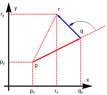
From the above figure, we can observe that in order for the points p, q and r need to be traversed in the same order in a counterclockwise direction, the cross product of the vectors pq and qr should be in direction out of the plane of the screen i.e., it should be positive.

The above result is being calculated by the orientation() function.

Thus, we scan over all the points rrr and find out the point qqq which is the most counterclockwise relative to ppp and add it to the convex hull. Further, if there exist two points(say iii and jjj) with the same relative orientation to ppp, i.e. if the points iii and jjj are collinear relative to ppp, we need to consider the point iii which lies in between the two points ppp and jjj. For considering such a situation, we've made use of a function inBetween() in the current implementation. Even after finding out a point qqq, we need to consider all the other points which are collinear to qqq relative to ppp so as to be able to consider all the points lying on the boundary.

Thus, we keep on including the points in the hull till we reach the beginning point.

The following animation depicts the process for a clearer understanding.

The Graham Scan Algorithm

The method works as follows. Firsly we select an initial point(bmbmbm) to start the hull with. This point is chosen as the point with the lowest y-coordinate. In case of a tie, we need to choose the point with the lowest x-coordinate, from among all the given set of points. This point is indicated as point 0 in the animation. Then, we sort the given set of points based on their polar angles formed w.r.t. a vertical line drawn throught the intial point.

This sorting of the points gives us a rough idea of the way in which we should consider the points to be included in the hull while considering the boundary in counter-clockwise order. In order to sort the points, we make use of orientation function which is the same as discussed in the last approach. The points with a lower polar angle relative to the vertical line come first in the sorted array. In case, if the orientation of two points happens to be the same, the points are sorted based on their distance from the beginning point(bmbmbm). Later on we'll be considering the points in the sorted array in the same order. Because of this, we need to do the sorting based on distance for points collinear relative to bmbmbm, so that all the collinear points lying on the hull are included in the boundary.

But, we need to consider another important case. In case, the collinear points lie on the closing(last) edge of the hull, we need to consider the points such that the points which lie farther from the initial point bmbmbm are considered first. Thus, after sorting the array, we traverse the sorted array from the end and reverse the order of the points which are collinear and lie towards the end of the sorted array, since these will be the points which will be considered at the end while forming the hull and thus, will be considered at the end. Thus, after these preprocessing steps, we've got the points correctly arranged in the way that they need to be considered while forming the hull.

Now, as per the algorithm, we start off by considering the line formed by the first two points(0 and 1 in the animation) in the sorted array. We push the points on this line onto a stackstackstack. After this, we start traversing over the sorted pointspointspoints array from the third point onwards. If the current point being considered appears after taking a left turn(or straight path) relative to the previous line(line's direction), we push the point onto the stack, indicating that the point has been temporarily added to the hull boundary.

This checking of left or right turn is done by making use of orientation again. An orientation greater than 0, considering the points on the line and the current point, indicates a counterclockwise direction or a right turn. A negative orientation indicates a left turn similarly.

Now, as per the algorithm, we start off by considering the line formed by the first two points(0 and 1 in the animation) in the sorted array. We push the points on this line onto a stackstackstack. After this, we start traversing over the sorted pointspointspoints array from the third point onwards. If the current point being considered appears after taking a left turn(or straight path) relative to the previous line(line's direction), we push the point onto the stack, indicating that the point has been temporarily added to the hull boundary.

This checking of left or right turn is done by making use of orientation again. An orientation greater than 0, considering the points on the line and the current point, indicates a counterclockwise direction or a right turn. A negative orientation indicates a left turn similarly.

If the current point happens to be occuring by taking a right turn from the previous line's direction, it means that the last point included in the hull was incorrect, since it needs to lie inside the boundary and not on the boundary(as is indicated by point 4 in the animation). Thus, we pop off the last point from the stack and consider the second last line's direction with the current point.

Thus, the same process continues, and the popping keeps on continuing till we reach a state where the current point can be included in the hull by taking a right turn. Thus, in this way, we ensure that the hull includes only the boundary points and not the points inside the boundary. After all the points have been traversed, the points lying in the stack constitute the boundary of the convex hull.