Return to computing page for the first course APMA0330
Return to computing page for the second course APMA0340
Return to computing page for the fourth course APMA0360
Return to Mathematica tutorial for the first course APMA0330
Return to Mathematica tutorial for the second course APMA0340
Return to Mathematica tutorial for the fourth course APMA0360
Return to the main page for the course APMA0330
Return to the main page for the course APMA0340
Return to the main page for the course APMA0360
Introduction to Linear Algebra with Mathematica
One of the main issues of harmonic analysis is a possibility of
restoring a function f from the ordered list of its Fourier coefficients, which we denote as | f ≫. Another closely related problem asks for determination of functions f from a given discrete data ∣∙≫. It turns out that synthetization of analog signal f(x) from the discrete data | f ≫ is an
ill-posed problem. Therefore, practical implementation of Fourier series may require a regularization, which is related to the scrutiny of
convergence of Fourier series. This topic is known as classical harmonic analysis, a branch of pure mathematics---it is discussed further in section on global convergence and in section devoted to Cesàro summation.
Historically, Fourier series was the first example of expansion of a function
with respect to eigenfunctions corresponding to a Sturm--Liouville problem.
Before Fourier's discovery,
Taylor series were mostly in use; however, their expansions require utilization of uniform and absolute convergence inside the disk, and pointwise convergence on its boundary. Taylor's series coefficients
are defined locally by derivatives evaluated at one single point---the center of convergence, so only
infinitesimal information is used for their determination. In opposite,
eigenfunction expansions are based on the integration over whole interval.
This caused development of another methods: 𝔏² convergence, summability, and the the Cesàro mean.
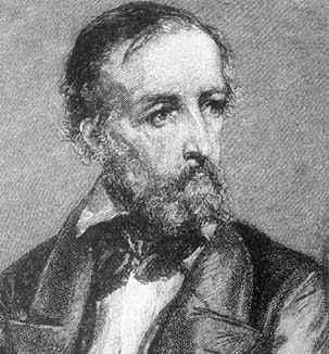
In 1873, the German mathematician Paul du Bois-Reymond (1831--1889) showed that there exists a continuous function whose Fourier series diverges at a point. His example indicates that a continuous function cannot be recovered from its Fourier series expansion. However, this ill-posed problem later in 1900 was solved by Lipót Fejér (1880--1956) who used Cesàro summability method to confirm uniform convergence of Fourier partial sums for a continuous periodic function. He also proved that if a trigonometric series converges to an integrable function, it must be its Fourier series.
Example 1:
We consider a 2π-periodic function whose Fourier series diverges. This function was constructed by Lipót Fejér in 1900.
Kolmogorov, A., Une serie de Fourier--Lebesgue divergente presque partout, Fundamenta Mathematicae, 1923, 4, 324--328.
■
This section is about some sufficient conditions that guarantee pointwise convergence of (formal) Fourtier series S[f] to f(x) either pointwise or uniformly.
There are known many conditions that assure convergence of Fourier series to the generating it function. However, we discuss only two important tests, known after Dirichlet and Dini, that provide pointwise convergence. If a function satisfies a Hölder condition, then its Fourier series converges uniformly.
Periodic Functions
There is a natural connection between 2ℓ-periodic functions on ℝ like the exponentials ejπθ/ℓ, functions on an interval of length 2ℓ, and functions on
the unit circle, which we denote as 𝕋 (because it is a one-dimensional torus). This connection arises as follows.
A point on the unit circle takes the form ejπθ/ℓ, where j is the imaginary unit on the complex plane ℂ so j² = −1, and θ is a real number
that is unique up to integer multiples of 2ℓ. If F is a function on the circle 𝕋 = ℝ/(2ℓℕ), then we may define for each real number θ∈ℝ a function
\[
f (\theta ) = F \left( e^{{\bf j}\pi\theta /\ell} \right) .
\]
Observe that with this definition, the function f is periodic on ℝ of period 2ℓ, that is, f(θ + 2ℓ) = f(θ) for all θ∈ℝ. The integrability, continuity, and other smoothness properties of F are determined by those of f.
For instance, we say that F is integrable on the circle 𝕋 if f is integrable
on every interval of length 2ℓ. Also, F is continuous on the circle 𝕋 if f is periodic and continuous on ℝ, which is the same as saying that f is continuous on
any interval of length 2ℓ. Moreover, F is continuously differentiable if f
has a continuous derivative, and so forth. The function f is a periodic function with period 2ℓ if the following condition is true:
Since f has period 2ℓ, we may restrict it to any interval of length 2ℓ,
say [0, 2ℓ] or [−ℓ, ℓ], and still capture the initial function F on the circle 𝕋.
We note that f must take the same value at the end-points of the interval
since they correspond to the same point on the circle. Conversely, any
function on [−ℓ, ℓ] for which f(−ℓ) = f(ℓ) can be extended to a periodic
function on ℝ that can then be identified as a function on the circle.
In particular, a continuous function f on the interval [−ℓ, ℓ] gives rise to
a continuous function on the circle 𝕋 if and only if f(−ℓ) = f(ℓ). Roughly speaking, circle 𝕋 is introduced to please lazy people who tied to write "periodic function."
In conclusion, functions on ℝ that are 2ℓ-periodic, and functions on an
interval of length 2ℓ that take on the same value at its end-points, are
two equivalent descriptions of the same mathematical object, namely,
functions on the circle 𝕋. In this connection, we mention an item of notational usage. When
our functions are defined on an interval on the line ℝ, we often use x as
the independent variable; however, when these functions are defined on the circle 𝕋, we usually replace the variable x by θ, which is mostly
a matter of convenience.
Here T = 2ℓ is the period and «P.V.» abbreviates the Cauchy principle value. As usual, j denotes the imaginary unit vector in the positive vertical direction on the complex plane ℂ, so j² = −1. These coefficients are related via the Euler formula:
There are two standard notations to represent a complex conjugate: either with overline or with asterisk, so we utilize both.
Series \eqref{EqConverge.1}
is an example of an
expansion of f(x) with respect to eigenfunctions corresponding to a Sturm--Liouville problem (see section for detail). Since this problem contains periodic boundary conditions, this expansion reflects this property. Therefore, we will always assume that a function f(x) is periodically expanded to ℝ with the same period T = 2ℓ to match the periodicity condition: f(x) = f(x + T).
Since Fourier series S[f] of a function f(x) is an example of infinite series, its convergence (or justification) depends on a rule how its partial sums
approach a limit as N → ∞. Therefore, we need a compact formula for finite partial sums SN(f; x); fortunately, such formula is known and it is based on Fourier decomposition of the Dirac delta function.
We expand the delta-function into Fourier series, Using the Euler--Fourier formulas, we get
for a smooth function f(x). This kind of convergence is abbreviated as δN ⇀ δ to indicate the weak convergence.
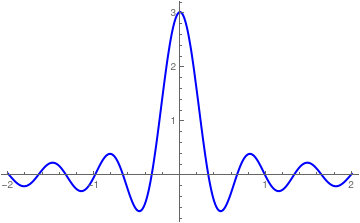
Actually there is a neat formula for the partial sum δN(x). It is called the Dirichlet kernel after the German scientist who first dicovered it in 1824.
Lemma 1:
The following trigonometric identity holds:
The denominator in the Dirichlet kernel \eqref{EqFourier.4} can vanish and hence this expression holds at the points, where it is not well-defined, according to L'Hôpital's rule.
Lemma 3:
The Dirichlet kernel possesses the following properties.
Before we get into the topic of convergence, we need to define some classes of functions that are suitable for Fourier expansions and wide enough to include the majority of practical applications. First, we extend the set of continuous functions on the interval [−ℓ, ℓ], which is usually denoted as ℭ[−ℓ, ℓ]. The set of periodic continuous functions is denoted by ℭ[𝕋] that includs continuous functions on [−ℓ, ℓ] subject to the periodicity condition:
f(−ℓ) = f(ℓ). We need this vector space ℭ[𝕋] because a Fourier series S[f] defines a periodic function indenedently whether the generating function f is periodic or not.
Correspondingly, the vector space of functions that have m first continuous derivatives on the closed interval [−ℓ, ℓ] is denoted by ℭm[−ℓ, ℓ]. Its subspace of periodic functions is denoted as ℭm[𝕋]. Between these two spaces, ℭ1[−ℓ ℓ] ⊂ ℭ[−ℓ, ℓ], there is another important space of absolutely continuous functions, denoted by AC[−ℓ, ℓ]. Recall that function f is called absolutely continuous if there exists a Lebesgue integrable function g on [−ℓ, ℓ] such that
where the supremum is taken over every finite partition P = { 𝑎 = x0 , x1, … , xn = b } of interval [𝑎, b] such that xi ≤ xi+1 for all n indices.
If f is differentiable and its derivative is Riemann-integrable, its total variation is the vertical component of the arc-length of its graph, that is,
\[
V_a^b (f) = \int_a^b \left\vert f' (x) \right\vert {\text d} x .
\]
According to Boris Golubov, a bounded variation functions of a single variable were first introduced by Camille Jordan, in the paper (1881) dealing with the convergence of Fourier series (Jordan, Camille (1881), "Sur la série de Fourier" [On Fourier's series], Comptes rendus hebdomadaires des séances de l'Académie des sciences, 92: 228–230).
Lemma (Jordan decomposition):
Every function of bounded variation on a finite closed interval is a difference of two bounded monootonic (nondecreasing) functions.
Recall that thetotal variation of functionf is defined to be
Thus, f is of bounded variation on [𝑎, b] if and only if Vb𝑎(f) is bounded on [𝑎, b]. Furthermore, given any function of bounded variation f on [𝑎, b], we may rewrite it as a difference of two monotonic functions:
Observe that \( f^{+} (x) = \tfrac{1}{2} \left[ V_a^b (f)(x) + f(x) \right] \) and \( f^{-} (x) = \tfrac{1}{2} \left[ V_a^b (f)(x) - f(x) \right] \)
are both monotone increasing functions. That is, a function is of bounded variation if and only if it is the difference of two monotonicaly increasing functions.
The set of all functions of bounded variabtion is usually denoted as BV[𝑎, b]. A BV function may have discontinuities, but at most countably many.
One of the most important aspects of functions of bounded variation is that they form an algebra of discontinuous functions whose first derivative exists almost everywhere.
We need to consider piecewise continuous functions that consist of finite number of continuous pieces. We say that f(x) has a jump discontinuity at x = 𝑎 if the limit of the function from the left, \( \lim_{t\uparrow a} f(t) , \) denoted \( f(a-0) \ \mbox{ or }\ f(a^{-}) \) and the limit of the function from the right, \( \lim_{t\downarrow a} f(t) , \) denoted \( f(a+0) \ \mbox{ or }\ f(a^{+}) , \) both exist and \( f(a+0) \ne f(a-0) . \) A function
f(x) is called piecewise continuous on an interval [𝑎, b], if it is continuous on [𝑎, b] except for at most finitely many points \( x_1 , x_2 , \ldots , x_n \) at each of them the function has both the left-hand and right-hand limits: \( f(x_k -0) \ \mbox{ and }\ f(x_k +0) , \quad k=1,2,\ldots , n . \) Now we give the formal definition.
Let 𝑎 and b be real numbers such that 𝑎 < b. A function \( f\, : \, [a,b] \mapsto \,\mathbb{R} \) is said to be piecewise continuous on \( [a,b] \)
if the following conditions are satisfied:
there exists a finite set \( \{ x_1 , x_2 , \ldots , x_n \} \subset (a, b) \) such that \( x_1 < x_2 < \cdots < x_n \) and f is continuous and monotone on each subinterval
\[
\lim_{x\downarrow a} f \left( x \right) , \quad \lim_{x\uparrow x_k} f\left( x \right) , \quad \lim_{x\downarrow x_k} f\left( x \right) ,\quad k=1,2,\ldots , n-1, \quad \lim_{x \uparrow b} f\left( x \right) .
\]
A function \( f\, : \, \mathbb{R} \mapsto \,\mathbb{R} \) is piecewise continuous on \( \mathbb{R} , \) if it is piecewise continuous on every finite subinterval of \( \mathbb{R} . \)
Example 5:
The function
\[
f(x) = \begin{cases} 2x , & \ \mbox{ if } 0 < x < 1, \\
1, & \ \mbox{ if } 1 < x < 2, \end{cases}
\]
is piecewise continuous on [0,2], but not continuous on [0,2].
Next, we plot partial sums along with the given function.
Fourier approximation with 10 terms
Fourier approximation with 20 terms
Fourier approximation with 100 terms
■
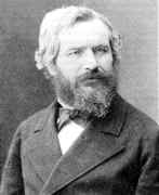
The first sufficient conditions for the pointwise convergence of the Fourier series were discovered by a German mathematician Johann Peter Gustav Lejeune Dirichlet (1805--1859). A function that satisfies the Dirichlet conditions is also called piecewise monotone. Such functions must have right and left limits at each point of discontinuity. We prove the corresponding theorem in convergence section.
is the Fourier series for a piecewise continuous function f(x) over the interval [−ℓ, ℓ]. If its derivative f'(x) is piecewise continuous on the interval \( [- \ell , \ell ] \) and has both a left- and right-hand derivative at each point in this interval, then F(x) is pointwise convergent for all x ∈ [−ℓ, ℓ]. The relation \( F(x) = f(x) \) holds at all points x ∈ [−ℓ, ℓ], where f(x) is continuous. If x = 𝑎 is a point of discontinuity of f, then
\[
F(x) \,=\, \frac{f(a+0)+ f(a-0)}{2} ,
\]
where \( f(a-0) = f(a^{-}) = \lim_{t\uparrow a} f(t) \) and \( f(a+0) = f(a^{+}) = \lim_{t\downarrow a} f(t) \) denote the left- and right-hand limits, respectively. ⧫
Since the class of continuous functions C[−ℓ, ℓ] contains functions that are different from their corresponding sum-Fourier series, we consider its subclass containing so called piecewise smooth functions.
We say that f(x) is piecewise smooth on some interval if
the interval can be broken up into a finite number of pieces (or sections) such
that in each piece the function f(x) is continuous and its derivative df/dx is also continuous. The function f(x) may not be continuous, but the only kind of discontinuity allowed
is a finite number of jump discontinuities.
If derivatives in the condition above are replaced by weaker condition so that function f is piecewise monotonic, then such function is said to satisfy the Dirichlet conditions. A function \( f\, : \, \mathbb{R} \mapsto \,\mathbb{R} \) is piecewise smooth on \( \mathbb{R} , \) if it is piecewise smooth on every finite subinterval of \( \mathbb{R} . \) The tangent
function is not piecewise smooth because its discontinuity is of infinite jump. On the other hand, the function sin(1/x) is not piecewise continuous because it has infinite number of maxima and minima in the neighborhood of the origin.
A real-valued function f defined on an interval [𝑎, b] is called piecewise smooth on it if it is piecewise continuous and its derivative is piecewise continuous.
Example 6:
Let f(x) = |sin(x)| be the absolute value of the sine function on the interval |−π, π|. This function is continuous on any subinterval of the real axis ℝ. Its derivative is piecewise continuous:
\[
f'(x) = \begin{cases}
\phantom{-}\cos x , & \ \mbox{ if }\quad 0 < x < \pi , \\
-\cos x , & \ \mbox{ if }\quad -\pi < x < 0 .
\end{cases}
\]
However, \( f(x) = |x|^{1/2} = \sqrt{|x|} \) is continuous on [-1,1], but it is not piecewise smooth on [-1,1] because we can break the interval [-1,1] into two subintervals [-1, 0} and (0, 1] on each of these the given function has no a bounded derivative.
■
as N → ∞ for every fixed x∈[−ℓ, ℓ].
It turns out that not every integrable (in Riemann sense, 1855) function possesses a convergent Fourier series. in 1923, Andrew Kolmogorov gave an example of a function from 𝔏¹ with an almost everywhere divergent Fourier series.Soon after, in 1926, he proved another example of Fourier series that diverges at every point. Some function have convergent Fourier series that have limiting values different from generating Fourier series. We denote the relation between a (periodic) function f(x) and its Fourier series as
This relation indicates that the Fourier coefficients are evaluated according to the Euler--Fourier formulas.
The first convergence theorem was proved in 1829 by the German
mathematician Peter Gustav Lejeune Dirichlet (1805--1859). Its proof is based on application of the second mean value theorem. It provides sufficient conditions for Fourier series to comverge pointwise without requirement on existence of a derivative of function f(x).
Second mean value Theorem:
Let g(x) be a bounded, increasing real valued function defined on the interval [𝑎,b], that is continuous at 𝑎 and b; and f(x) a Riemann integrable function on [𝑎,b]. Then there exists a real number c∈[𝑎,b] such that
\[
\int_a^b g(x)\,f(x)\,{\text d} x = g(a+0) \int_a^c f(x)\,{\text d} x + g(b-0) \int_c^b f(x)\,{\text d} x .
\]
There are known other sufficient conditions that guarantee pointwise convergence of a Fourier series; however, we start with a classical statement credited to Dirichlet.
Theorem (Dirichlet):
Let f(x) be a periodic function with period T = 2ℓ
and satisfy the following conditions (that are usually referred to as the
Dirichlet conditions):
f(x) must be of bounded variation (which means that the function has finite number of local maximum and minimum points and it monotonically increases/decreases between them) in any given bounded interval;
f(x) must have a finite number of discontinuities in any given bounded interval, and the discontinuities cannot be infinite.
The Dirichlet theorem assures that the Fourier series
\( \frac{a_0}{2} + \sum_{k\ge 1} a_k \cos \frac{k\pi x}{\ell} + b_k \sin \frac{k\pi x}{\ell} \) converges to
f(x) at all points where f is continuous inside the interval (−ℓ, ℓ);
\( \displaystyle \frac{f(-\ell +0) + f(\ell -0)}{2} \)
at endponts.
The absolutely integrability condition is a sufficient condition to guarantee existence of Fourier coefficients. The last two conditions of Dichlet's theorem are imposed to apply the second mean value theorem:
In section on Fourier series, a class of functions,
called piecewise smooth, was introduced. Such functions satisfy the Dirichlet conditions.
Riemann-Lebesgue lemma:
Let f(x) ∈ 𝔏[𝑎, b] be absolutely integrable function on the interval [𝑎. b]. Then
Allowing n → ∞, we obtain the stated limit. A similar argument holds for the sine.
Suppose now that f(x) ∈ 𝔏[𝑎. b]. Given ε > 0, we can find a polynomial p(x) such that
\( \int_a^b \left\vert f(x) - p(x) \right\vert {\text d}x \le \varepsilon. \) Now,
Notice that in the integral over [δ, π], the integrand is an integrable function and hence the Riemann-Lebesgue lemma guarantees that it approaches zero as n → ∞.
Lemma 7:
If function ψ(x) is monotonic in an interval [0, δ], for some positive δ, then
Since the function \( \displaystyle \frac{\sin (mz)}{z} \) is integrable on the interval [0, δ] for any δ, we can apply the second mean value theorem and obtain
In order to prove the Dirichlet theorem, we need to show that the difference Sn(x) − f(x) approaches zero as n → ∞. Let us fix x and consider the function
has no singulariry in a neighborhood of the origin, it is integrable over [0, δ]. Hence, by the Riemann--Lebesgue lemma, the latter integral → 0 as n → ∞. Application of the second mean value theorem provides the required result because ψ(0) = 0.
Lemma 8:
Let f be a continuous periodic function. If its Fourier series converges absolutely, then the Fourier series converges to f uniformly.
; ⧫
Theorem 3:
For piecewise smooth f(x), the Fourier series of f(x) is continuous
and converges to f(x) for −ℓ ≤ x ≤ ℓ if and only if f(x) is
continuous and f(−ℓ) = f(ℓ).
⧫
Theorem 4:
A Fourier series for a 2ℓ-periodic function f(x) that is continuous can be differentiated term by
term if its derivative f'(x) satisfies the Dirichlet conditions.
⧫
Using this definition, he improved the Dirichlet theorem.
Theorem 6 (Dirichlet--Jordan criterion):
Suppose that f(x) is of bounded variation over interval [−ℓ, ℓ]. Then
at every point x0, the Fourier series S[f] converges to the value \( \displaystyle \tfrac{1}{2} \left[ f(x_0 +0) + f(x_) -0) \right] \) ; in particular, the Fourier series S[f] converges to f(x) at every point of continuity of f;
if further f is continuous at every point of a closed interval [𝑎, b], then its Fourier series S[f] converges uniformly in [𝑎, b].
The proof of this theorem follows from the Dirichlet theorem and the following lemma.
Since the Direchlet kernel is an even function (as sume of cosine functions), the partial Fourier sum can be written as
Note that a constant K is independenyt on C, N, and δ. This completes the proof
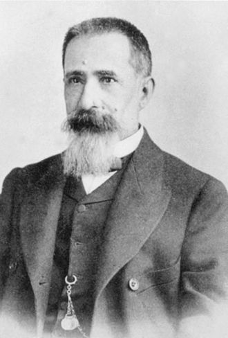
The following theorem was proved in 1880 by an Italian mathematician Ulisse Dini (1845--1918).
Theorem 6 (Dini's criterion):
Suppose that a function f(x) ∈ 𝔏[−ℓ, ℓ] is absolutely integrable, and let
ψ(t) = f(x + t) + f(x −t) −2f(x) for a fixed x. If the integral
We split the integral into the regions where |y| < δ and δ < |y| < 2π. For latter domain of integration, we have
\( \frac{1}{|\sin (y/2) |} \le M \) for some positive constant M. Then
Ulisse Dini
Observe that for Dini’s theorem to hold, it is in fact enough to have that there existconstants H > 0 and α ∈ (0, 1] such that that whenever |y ≤ 2ℓ, we have
\[
| f(x-y) - f(y)| \le H \left\vert y \right\vert^{\alpha} .
\]
Such functions are called α-Hölder continuous. Note that if function f has a continuous derivative, then f is automatically 1-Hölder (also known as Lipschitz).
The smoothness of the function drastically affects the rate of decrease of the Fourier coefficients: the smoother the function the more rapidly its Fourier coefficient decreease. The study of pointwise convergence of Fourier series is largely the study of the interplay between assumprions of smoothness and conclusions about convergence.
Order of Decay of Fourier Coefficients
We investigate the interplay between the smoothness of a function and the decay of its Fourier coefficients.
Let us consider a function f(x) having N continuous derivatives on [−ℓ, ℓ]. The integrals in Euler--Fourier formulas \eqref{EqFourier.2} and \eqref{EqFourier.4} can be integrated by parts N times. Taking one coefficient, say 𝑎k, and integrate by parts twice, we obtain
So we see that if function f(x) has one periodic derivative and the second derivative is integrable, the Fourier coefficients decay as 1/k². Clearly, this process can be continued until the N-th differential appears in the integral, but useful information can be greened from these expressions.
Theorem 6:
If a periodic function f(x) is continuous and has continuous periodic derivatives up to the (N−1)-st order and if its N-th derivative is integrable on interval [−ℓ, ℓ], then its Fourier coefficients can be estimated by
Example 11: ?????????????
We consider the power function \( f(x) \left( x^2 - \ell^2 \right)^2 . \) Expanding it into Fourier series, we get
\[
\left( x^2 - \ell^2 \right)^2 =
\]
■
Theorem 7:
Let f(x) ∈ ℭn[−ℓ, ℓ], that it has n continuous derivatives, and have period 2ℓ, that is, f(−ℓ) = f(ℓ), f'(−ℓ) = f'f(n)(−ℓ) = f(n)(ℓ). Suppose further that its n-th derivative is a Lipschitz function of order α, 0 < α ≤ 1. The the Fourier coefficients of f satisfy the inequalities
Corollary:
Let f(x) be continuous and periodic on the interval [−ℓ, ℓ], f(−ℓ) = f(ℓ), and suppose that the Fourier series of f(x) converges uniformly there. Then it converges to f(x).
Corollary:
If f(x) is continuous on the interval [−ℓ, ℓ], f(−ℓ) = f(ℓ), and all its Fourier coefficients are zeroes, then f(x) ≡ 0.
Theorem 10:
Let f(x) be a continuous periodic function in [−ℓ, ℓ], f ∈ ℭ[𝕋]. If the Fourier series S[f] converges uniformly, then it converges to f(x).
If Fourier series \eqref{EqConverge.1} converges uniformly, it will converge to a continuous function of period 2ℓ. Let us call this sum
g(x):
Hence their difference f(x) − g(x) is orthogonal to the complete set of trigonometric functions. This leads to
f(x) ≡ g(x).
Corollary 10:
Let f(x) be continuous and periodic in [−ℓ, ℓ] and have Fourier coefficients 𝑎k, bk according to Eq.\eqref{EqFourier.5T}. If \( \displaystyle \sum_{k\ge 1} \left( \left\vert a_k \right\vert + \left\vert b_k \right\vert \right) \) converges, then the Fourier series of f converges absolutely and uniformly to f(x), x∈[−ℓ, ℓ]. Similarly, if \( \displaystyle \sum_{\nu =-\infty}^{+\infty} \left\vert \hat{f}(\nu ) \right\vert < \infty , \) then the Fourier series S[f] converges absolutely and uniformly.
it follows from the Weierstrass M-test that the Fourier series converges uniformly and absolutely. By the previous theorem, it converges to f(x).
Example 12: ?????????????
End of Example 4
Now we take advantage of smoothness to proof uniform convergence of Fourier series.
Theorem 11:
Let f ∈ ℭ²[𝕋], with period 2ℓ. Then the Fourier series of f(x) converges uniformly and absolutely to f(x).
Theorem above can be improved.
Theorem 12:
Let f be a periodic continuous function of period 2ℓ, and have a derivative that is piecewise continous in [−ℓ, ℓ]. Then the Fourier series of f converges uniformly and absolutely in [−ℓ, ℓ] to f(x).
Integrating by parts, we find the coefficient Fourier:
Hence \( \displaystyle \sum_{k\ge 1} \left\vert a_k \right\vert < \infty . \) A similar argument shows that
\( \displaystyle \sum_{k\ge 1} \left\vert b_k \right\vert < \infty . \) The theorem now follows by Corollary 10.
Note that the conclusion of the previous theorem is valid when the derivative of function f belongs to 𝔏²[−ℓ, ℓ].
It is well known that the Fourier series of a
continuous function is not necessarily uniformly convergent in
an interval of continuity of the sum-function. However, if, in
addition to being continuous, the function is also of bounded
variation then it is known that the Fourier series is uniformly
convergent in the interval of periodicity. This is the so-called
Jordan criterion for uniform convergence,
A second criterion for uniform convergence is the Dini-
Lipschitz condition. If for 0 < |t| < 1
\[
| f(x+t) - f(x) | < \frac{K}{\left( -\log |t| \right)^{1+\alpha}} , \qquad K, \alpha > 0 ,
\]
then the Fourier series of f ( x ) converges uniformly.
Let f be a periodic function on [−ℓ, ℓ], let t be some point and let δ be a positive number. We define the local modulus of continuity at the point t by
Theorem 2 (Dini's test):
Suppose that f is continuous in a closed interval [𝑎, b] and let ω(δ) be its modulus of continuity there. If ω(δ)/δ is integrable near δ = 0, and if the integrals
P.G.L. Dirichlet, "Sur la convergence des séries trigonometriques qui servent à réprésenter une fonction arbitraire entre des limites données"
Journal für die reine und angewandte Mathematik, 1829,
Volume: 4, pages 157-169.
ISSN: 0075-4102; 1435-5345/e
Duoandikoetxea, J. Fourier Analysis (Graduate Studies in Mathematics), American Mathematical Society, Providence, RI, 2000.
Golubov, B.I., Dini criterion, Encyclopedia of Mathematics, 2001, EMS Press
Hewitt, E. and Hewitt, R.E., The Gibbs--Wilbraham phenomenon: An episode in Fourier analysis, Archive for History of Exact Science, 1979, Vol. 21, No. 2, pp. 129--160.
C. Jordan, "Sur la série de Fourier" C.R. Acad. Sci. Paris , 92 (1881) pp. 228–230.
Rhatia, R. Fourier Series, Mathematical Association of America, Washington DC, 2005.
Zygmund, A., Trigonometric Series, Volumes I and II combined, Third edition, Cambridge University Press, 2003. ISBN-13 : 978-0521890533
Return to Mathematica page
Return to the main page (APMA0360)
Return to the Part 1 Basic Concepts
Return to the Part 2 Fourier series
Return to the Part 3 Integral Transformations
Return to the Part 4 Parabolic Differential Equations
Return to the Part 5 Hyperbolic Differential Equations
Return to the Part 6 Elliptic Equations
Return to the Part 7 Numerical Methods
a.png)
b.png)
c.png)