This section expands Picard's iteration process to
systems of ordinary differential equations in normal form (when the derivative is isolated). Picard's iterations for a single
differential equation \( {\text d}x/{\text d}t = f(t,x)
\) was considered in detail in the
first tutorial (see
section for reference). Therefore, our main interest would be to apply Picard's iteration to systems of first order ordinary differential equations in normal form (which means that the highest derivative is isolated)
This explicit notation cannot be called compact and informative. Hence, we introduce n-dimensional vectors of unknown variables and slope functions in order to rewrite the above system in compact form. So
the system of differential equations can be written in vector form
are n-column vectors. Note that the above system of equations contains
n dependent variables \( x_1 (t), x_2 (t) , \ldots ,
x_n (t) \) while the independent variable is denoted by t,
which may be associated with time. In engineering and physics, it is a custom
to follow Isaac Newton and denote a derivative with respect to time variable t by dot:
\( \dot{\bf x} = {\text d}{\bf x} / {\text d} t. \)
When input function f satisfies some general conditions (usually
required to be Lipschitz
continuity in the dependent variable \( {\bf x} \) ), then
Picard's iteration converges to a solution of the Volterra integral equation
in some small neighborhood of the initial point. Thus, Picard's iteration is
an essential part in proving existence of solutions for the initial value
problems.
Note that Picard's iteration is not suitable for numerical
calculations. The reason is not only in slow convergence, but
mostly it is impossible, in general, to perform explicit integration to
obtain
next iteration. Although in case of polynomial input function, integration
can be performed explicitly (especially, with the aid of a computer algebra
system), the number of terms quickly grows as a snow ball. While we know that the resulting series converges eventually to the true solution, its range of convergence is too small to keep many
iterations. In another section, we show how
to bypass this obstacle.
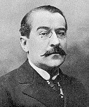
Charles Picard
If an initial position of the vector \( {\bf x} (t) \)
is known, we get an initial value problem:
where \( {\bf x}_0 \) is a given column vector.
Many brilliant mathematicians participated in proving the existence of a
solution to the given initial value problem more than 100 years ago. Their
proof was based on what is now called the Picard's iteration, named after the
French mathematician Charles Émile Picard (1856--1941) whose theories did much to advance
research in analysis, algebraic geometry, and mechanics.
The Picard procedure is actually a practical extension of the Banach fixed point theorem, which is applicable to continuous contractive function. Since any differential equation involves an unbounded derivative operator, the fixed point theorem is not suitable for it. To bypass this obstacle, Picard suggested to apply the (bounded) inverse operator L-1 to the derivative one \( \texttt{D} . \) Recall that the inverse \( \texttt{D}^{-1} , \) called in mathematical literature as «antiderivative», is not an operator because it assigns to every input-function infinite many outputs. To restrict its output to a single one, we consider the differential operator on the set of functions (which becomes a vector space only when the differential equation and the initial condition are all homogeneous) with a specified initial condition f(x0) = y0. So the derivative operator on this set of functions we denote by L, and its inverse is a bounded integral operator.
The first step in deriving Picard's iterations is to rewrite the
given initial value problem in equivalent (this is true when the slope function f is continuous in Lipschitz sence) form as Volterra integral equation of second kind:
This integral equation is obtained upon integration of both sides of the
differential equation \(
{\text d}{\bf x} / {\text d} t = {\bf f}(t, {\bf x}), \) subject to the initial condition.
The equivalence follows from the Fundamental Theorem of Calculus. It suffices to find a continuous function \( {\bf x}(t) \)
that satisfies the integral equation within the interval \( t_0 -h < t < t_0 +h , \) for
some small value \( h \) since the right hand-side (integral) will be continuously differentiable in \( t . \)
Now we apply a technique known as Picard iteration to construct the required solution:
The initial approximation is chosen to be the initial value
(constant): \( {\bf x}_0 (t) \equiv {\bf x}_0
.\) (The sign ≡ indicates the values are identically
equivalent, so this function is the constant).
When input function f(t, x) satisfies some (sufficient)
conditions, it can be shown that this iterative sequence converges to
the true solution uniformly
on the interval \( [t_0 -h, t_0 +h ] \) when
h is small enough.
Actually, the necessary and sufficient conditions for existence of a solution
to a vector initial value problem are still waiting for their discovery.
Of course, we can differentiate the recursive integral relation to obtain a sequence of the initial value problems
that is equivalent to the original recurrence \eqref{EqPicard.3}. However,this recurrence relation \eqref{EqPicard.4} involves the derivative operator
\( \texttt{D} = {\text d}/{\text d}t . \) Since \( \texttt{D} \) is an unbounded operator, it is not possible to prove convergence of iteration procedure \eqref{EqPicard.4}. On the other hand, the convergence of \eqref{EqPicard.3} involving a bounded integral opeprator can be accomplished directly (see Tutorial I).
If we start with the initial condition ϕ0 = 1, we almost immediately come to a problem of explicit integration. Indeed, we calculate first the few terms:
To apply Picard's method, we convert the given initial value problem to the system of differential equations upon introducing auxiliary dependent variables:
The second component, ϕ2, remains the same with
every iteration. This component is used to generate the first
component, ϕ1, as well. As such, every following iteration will be the
same, and the true solution becomes
where dot stands for the derivative with respect to time
variable t.
We integrate the pendulum equation above twice, and use initial condition
provided. We may try to apply Picard's iteration scheme
next term ϕ3(t) is impossible to determine, even for such powerful computer algebra system as Mathematica. We can bypass this obstacle by introducing auxiliary variables:
where d = 1 is the initial displacement and v =-1 is the initial
velocity. For simplicity, we choose the following numerical values of
parameters: η = 3 and ε = 1. First, we convert the given problem
to a system of first order differential equations
■
Example 8:
■
Example:
**DESCRIPTION OF PROBLEM GOES HERE**
This is a description for some MATLAB code. MATLAB is an extremely
useful tool for many different areas in engineering