Part 2.2: Motivation

This section presents motivating examples to study systems of ordinary differential equations (ODE for short),

\[ \begin{cases} \dot{y}_1 &= f_1 \left( y_1 , y_2 , \ldots , y_n , t \right) , \\ \dot{y}_2 &= f_2 \left( y_1 , y_2 , \ldots , y_n , t \right) , \\ \cdots & \qquad \cdots \\ \dot{y}_n &= f_n \left( y_1 , y_2 , \ldots , y_n , t \right) , \\ \end{cases} \]

or in vector form

\begin{equation} \label{EqMotiv.1} \dot{\bf y} = {\bf f} \left( {\bf y},t \right) , \end{equation}

where y(t) and f(y, t) are column-vectors:

\[ {\bf y} (t) = \begin{bmatrix} y_1 (t) \\ \vdots \\ y_n (t) \end{bmatrix} = \left[ y_1 (t), \ldots , y_n (t) \right]^{\mathrm{T}} , \qquad {\bf f}({\bf y}, t) = \begin{bmatrix} f_1 \left( y_1 , \ldots , y_n , t \right) \\ \vdots \\ f_n \left( y_1 , \ldots , y_n , t\right) \end{bmatrix} . \]

The system of differential equations \eqref{EqMotiv.1} occurs frequently in particular descriptions of physical phenomena from natural science. Autonomous systems have input function not containing t explicitly: f = f(y). With natural extension of known statements for a single differential equation, we present the following existence and uniqueness theorem.

Theorem: Consider the initial value problem

\begin{equation} \label{EqMotiv.IVP} \dot{\bf y} = {\bf f} \left( {\bf x},t \right) , \qquad \dot{\bf y}(0) = \dot{\bf y}_0 , \end{equation}

where y₀ ∈ ℝⁿ. Suppose that f : ℝⁿ → ℝⁿ is a continuously differentiable function. Then there exists a unique solution of the given initial value problem \eqref{EqMotiv.IVP}.

Here overdot stands for the derivative with respect to time variable, \( \dot{y} = {\text d}y/{\text d}t . \) http://homepages.math.uic.edu/~jan/mcs320/mcs320.pdf

Example 1: Consider the planar system of equations

\[ \begin{cases} \dot{x} = x^2 + y , \\ \dot{y} = y^2 + x . \end{cases} \]

To plot the direction field for the given system of equations, we ask Sage:

Each solution x = x(t), y = y(t) of the equation above satisfying the initial condition \[ x(0) > 0 , \qquad y(0) > 0 , \] cannot exist on an interval 0 ≤ t < ∞

In fact, the trajectory of any solution initiating in the first quadrant is contained in the first quadrant. So its global solution does not exist. ■

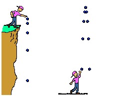
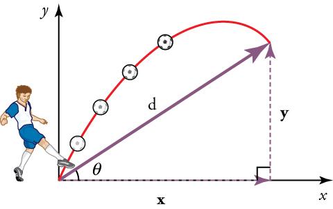
We start with motivating examples that you most likely saw in other courses.

Example 2: A projectile is an object upon which the only force acting is gravity, so the influence of air resistance is negligible. More realistic motion under drag force will be considered in the next example. Ballistics (Greek: βάλλειν, romanized: ba'llein, lit. 'to throw') or more precisely, projectile motion in a vacuum is a popular topics in physics at upper secondary schools and colleges. There are a variety of examples of projectiles. An object dropped from rest is a projectile; object that is thrown vertically upward is also a projectile. So we first consider a projectile that is thrown upward at an angle α to the horizontal line.


Vertical trajectories.		Projectile thrown upward at angle α to abscissa.

Its trajectory has a parabolic shape when the projectile of mass m is launched into a vacuum under angle α to horizontal axis (abscissa). The motionof the projectile is under the influence of gravity only. The position vector of the projectile at time t after firing is defined by the vector

\[ {\bf r} (t) = \left( x(t), y(t) \right) = x(t)\,{\bf i} + y(t)\,{\bf j} \]

and was set into motion with the initial velocity

\[ \left( v_0 \cos\alpha, v_0 \sin\alpha \right) = v_0 \cos\alpha\,{\bf i} + v_0 \sin\alpha\,{\bf j} . \]

The equations of motion are

\[ \begin{split} \ddot{x} &= 0 , \qquad x(0) = 0, \quad \dot{x}(0) = v\,\cos\alpha \\ \ddot{y} &= -g , \qquad y(0) =0, \quad \dot{y}(0) = v\,\sin\alpha , \end{split} \]

where g is the acceleration due to gravity. Solving these equations, we obtain

\[ \begin{split} x(t) &= v_0 t\,\cos\alpha , \\ y(t) &= v_0 t\,\sin \alpha - \frac{g\,t^2}{2} , \end{split} \]

One can eliminate t from the equations above and get \begin{equation*} y = \left( \tan\alpha \right) x - \frac{g\,\sec^2 \alpha}{2\,v_0^2} \, x^2 . \end{equation*} The equation above represents a quadratic function: thus, its graph is a parabola. Therefore, in the absence of air resistance, the path of the projectile is a parabola.

The time T taken by the projectile to reach the maximum height H, and the range R of the projectile are given by

\[ \begin{split} T &= \frac{v_0}{g}\,\sin\alpha , \\ H &= \frac{v_0^2}{2g}\,\sin^2 \alpha , \\ R &= \frac{v_0^2}{g}\,\sin (2 \alpha ) . \end{split} \]

Let (x_m, y_m) be coordinates of the vertex corresponding to the parabola solution curve, so y_m is the maximum height attained and x_m is the corresponding horizontal coordinate. \[ x_m = \frac{v_0^2}{2g} \,\sin \left( 2\alpha \right) , \qquad y_m = \frac{v_0^2}{2g} \,\sin^2 \alpha \]

de Alwise, T., Projectile motion with Mathematica, International Journal of Mathematical Education in Science and Technology, 2000, Vol. 31, No. 5, pp.749--755. doe: 10.1080/002073900434413
Benacka, I., Stubna, I., Ball launched against an inclined plane---an example of using recurrent sequences in school physics, International Journal of Mathematical Education in Science and Technology, 2009, Vol.40, No. 5, pp. 696--705.
Bose, S.K., Thoughts on projectile motion, American Journal of Physics, 1985, Vol. 53, No. 2, pp. 175
de Mestre, N., The Mathematics of Projectiles in Sport, Cambridge University Press, 2012, https://doi.org/10.1017/CBO9780511624032
Donnelly, D., The parabolic envelope of constant initial speed trajectories, American Journal of Physics, 1992, Vol. 60, No. 12, pp. 1149--1150.
Fernández-Chapou, J.L., Salas-Brito, A.L. and Vargas, C.A., An elliptic property of parabolic trajectories, American Journal of Physics, 2004, Vol. 72, pp. 1109--1110.
Hu, H., Yu, J., Another look at Projectile motion, The Physics Teacher, 2000, Vol. 38, No. 10, page 423.
Padyala, R., An alternative view of the elliptic property of a family of projectile paths, The Physics Teacher, 2019, Vol. 57, No. 9, pp376--377.
Sarafian, H., On projectile motion, The Physics Teacher, 1999, Vol. 37, No. 2, [[. 86--88.

Example 3: A particular practical interest is a situation when the projectile moves under gravity in a medium whose resistance is not negligible. The drag force acting on the projectile depends on many factors, including material of the projectile, its shape, speed, and some other parameters. Most of these factors are incorporated in the Reynolds number, which we denote by R_e to avoid confusion with "Re", which serves to identify a "real part" of a complex number (a standard notation for the Reynolds number is Re). The Reynolds number is the ratio of inertial forces to viscous forces within a fluid which is subjected to relative internal movement due to different fluid velocities. This number was introduced by Sir George Stokes (1819--1903), and popularized by Osborne Reynolds (1842--1912).

Since an accurate determination of the resistive force is very complicated, we concentrate our attention on a projectile having shape of a sphere. Fortunately, the dependents of the air resistive force acting on a ball is known and it depends on projectile's speed. For a sphere of radius r moving a fluid of density ρ and viscosity η, the drag force and the Reynolds number are

\[ \begin{split} F = 6\pi \eta\rho v \qquad \mbox{for} \quad R_e < 1, \\ R_e = 2r\rho v/\eta . \end{split} \]

For a ball with a density of 1 g/cm³, and using the value of ratio η/ρ = 0.15 cm²/sec for air, one finds utilization of a linear grad force appropriate when

\[ r \le 4 \times 10^{-3} \mbox{ cm}. \]

Spheres with this small of a radius would seem to be of little interest. For spheres with radii and speeds of practical interest a reasonable approximation to the drag force is

\[ F = \pi r^2 v^2 /4 \qquad \mbox{for} \quad 1 \ll R_e \le 10^5 . \]

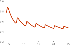
		The dependence of the drag force on velocity of a ball moving in air is well documented. Experiments measuring drag force dependence on the ball velocity were conducted by the faculty at MIT, which shows a complicated behavior. For small velocities, it is approximately linear, but then drag force starts closer to the quadratic function with speed increases. At large Reynolds numbers, we observe turbulence behind the ball. So when speed increases (and the Reynolds number exceeds 10⁵), the drag force declines and oscillates as shown in the figure. Such phenomena is observed in baseball and volleyball. f[t_, y_] = Sin[2.35ty]Cos[t + 1.0y];; s = NDSolve[{y'[t] == f[t, y[t]], y[0] == 1}, y, {t, 0, 30}]; Plot[Evaluate[y[t] /. s], {t, 3.9, 25}, PlotRange -> {0.2, 1}, PlotTheme -> "Web"]
Figure 1: Dependence of the drag force on ball's speed.		Mathematica code

Our next example is from mechanics and it requires the application of Euler--Lagrange equations for a conservative case:

\begin{equation} \label{EqMotiv.2} \frac{\text d}{{\text d}t}\,\frac{\partial {\cal L}}{\partial \dot{q}_i} \left( t, {\bf q}(t), \dot{\bf q}(t) \right) = \frac{\partial {\cal L}}{\partial q_i} \left( t, {\bf q}(t), \dot{\bf q}(t) \right) , \qquad i=1,2,\ldots n, \end{equation}

where q = (q₁, q₂, … , q_n) are generalized (canonical) coordinates and the Lagrangian is the difference between the kinetic and potential energy:

\begin{equation} \label{EqMotiv.3} {\cal L} = {\text K} - \Pi . \end{equation}

For a simple autonomous system \( \dot{\bf y} + {\bf f}({\bf y}) = 0, \) with K = \( \dot{\bf y}^2 = \dot{y}^2_1 + \cdots + \dot{y}^2_n \) and \( \Pi = {\bf f}^2 ({\bf y}) , \) we have

\[ \pi_y = \frac{\partial {\cal L}}{\partial \dot{\bf y}} = \left[ \frac{\partial {\cal L}}{\partial \dot{y}_1} , \ldots , \frac{\partial {\cal L}}{\partial \dot{y}_n} \right] = 2\,\dot{\bf y}, \qquad \frac{\partial {\cal L}}{\partial {\bf y}} = 2{\bf f}({\bf y}) \cdot {\bf f}' ({\bf y}) , \]

where π_y is the moment canonically conjugated to the variable y. The corresponding Hamiltonian is

\[ {\cal H} = {\mbox K} + \Pi = \pi_y \,\dot{\bf y} - {\cal L} = \dot{\bf y}^2 + {\bf f}^2 ({\bf y}) . \]

Example 4: As our running example of a differential equation, consider a pendulum. We have a mass attached to a string, subject to gravity. The variable is theta(t), the angle of deviation from the vertical position of the string, as a function in time. We start with modeling a simple pendulum, which consists of a body (bob) suspended from a fixed point (pivot) so that it can swing back and forth under the influence of gravity. We consider the simple pendulum that is characterized by the following assumptions:

The bob is free to move within a plane (so we consider only two-dimensional oscillations).
The system is conservative, so the pendulum rotates in a vacuum and friction in the pivot is negligible.
The bob of mass m is attached to one end of a rigid, but weightless rod of length ℓ, which is assumed to be constant during the pendulum motion. The other end of the rod (or rigid spring) is supported at the pivot.

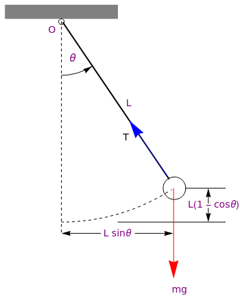
First, we illustrate with Sage the motion of the simple pendulum.

The modeling of the motion is greatly simplified when the given body (bob) is considered essentially as a point particle. The position of the bob is described by the angle θ between the rod and the downward equilibrium vertical position, with the counterclockwise direction taken as positive. The only force acting on the pendulum is the gravitational force m g, acting downward, where g denotes the acceleration due to gravity. The position of the bob can be determined in Cartesian coordinates as

\[ x = \ell \,\sin \theta , \qquad y = -\ell\,\cos\theta , \]

where the origin is taken at the pivot and the positive vertical direction is upward. Using \( {\cal L} = \mbox{K} - \Pi , \) the Lagrangian, which is the difference of the kinetic energy K and the potential energy Π of the system, we have

\[ \frac{\text d}{{\text d}t} \,\frac{\partial {\cal L}}{\partial \dot{\theta}} = \frac{\partial {\cal L}}{\partial \theta} . \]

With the kinetic energy expressed via the angular displacement θ

\[ \mbox{K} = \frac{m}{2} \left( \dot{x}^2 + \dot{y}^2 \right) = \frac{m}{2}\, \ell^2 \left[ \left( \dot{\theta} \,\cos\theta \right)^2 + \left( \dot{\theta} \,\sin \theta \right)^2 \right] = \frac{m}{2}\,\ell^2 \dot{\theta}^2 . \]

and the potential energy

\[ \Pi = mg \left( \ell + y \right) = mg\ell \left( 1- \cos \theta \right) , \]

we derive the corresponding derivatives

\[ \frac{\partial \mbox{K}}{\partial \dot{\theta}} = I_0 \dot{\theta} = m\ell^2 \dot{\theta} , \qquad \frac{\partial \Pi}{\partial \theta} = mgy = mg\ell \, \sin \theta . \]

Using these expressions, we obtain from the Euler--Lagrange equation \( \displaystyle \frac{\text d}{{\text d} t} \left( \frac{\partial {\cal L}}{\partial \dot{\theta}} \right) = \frac{\partial {\cal L}}{\partial \theta} , \) for the Lagrangian \( {\cal L} = \mbox{K} - \Pi , \) the pendulum equation in a vacuum:

\[ \ddot{\theta} + \left( g/\ell \right) \sin \theta =0 \qquad \mbox{or} \qquad \ddot{\theta} + \omega_0^2 \sin \theta =0 \qquad \left( \omega_0^2 = g/\ell \right) , \]

where \( \ddot{\theta} = {\text d}^2 \theta / {\text d}t^2 \) , \( \omega_0 = \sqrt{g/\ell} >0 ,\) and g is gravitational acceleration.

Now we consider a double pendulum, that consists of one pendulum attached to another. Consider a double bob pendulum with masses m₁ and m₂ attached by rigid massless wires of lengths ℓ₁ and ℓ₂. Further, let the angles the two wires make with the vertical be denoted θ₁ and θ₂, as illustrated in the figure to the left. Finally, let gravity acceleration be given by g. Then the positions of the bobs are given by

\begin{align*} x_1 &= \ell_1 \sin\theta_1 , \\ y_1 &= - \ell_1 \cos\theta_1 , \\ x_2 &= \ell_1 \sin\theta_1 + \ell_2 \sin\theta_2 , \\ y_2 &= - \ell_1 \cos\theta_1 - \ell_2 \cos\theta_2 . \end{align*}

The potential energy of the system is then given by

\begin{align*} \Pi &= m_1 g \left( \ell_1 + y_1 \right) + m_2 g \left( \ell_2 + y_2 \right) \\ &= m_1 g \ell_1 \left( 1 - \cos\theta_1 \right) + m_2 g \ell_2 \left( 1 - \cos\theta_2 \right) , \end{align*}

and the kinetic energy by

\begin{align*} \mbox{K} &= \frac{1}{2}\,m_1 v_1^2 + \frac{1}{2}\,m_2 v_2^2 \\ &= \frac{1}{2}\,m_1 \ell_1^2 \dot{\theta}^2_1 + \frac{1}{2}\,m_2 \left[ \ell_1^2 \dot{\theta}^2_1 + \ell_2^2 \dot{\theta}^2_2 + 2\ell_1 \ell_2 \dot{\theta}_1 \dot{\theta}_2 \cos \left( \theta_1 - \theta_2 \right) \right] . \end{align*}

The Lagrangian is then

\begin{align*} {\cal L} &= \mbox{K} - \Pi \\ &= \frac{1}{2} \left( m_1 + m_2 \right) \ell_1^2 \dot{\theta}_1^2 + \frac{1}{2} \,m_2 \ell_2^2 \dot{\theta}_2^2 + m_2 \ell_1 \ell_2 \dot{\theta}_1 \dot{\theta}_2 \cos \left( \theta_1 - \theta_2 \right) . \end{align*}

Performing calculations for one variable θ₁, we obtain

\begin{align*} \frac{\partial {\cal L}}{\partial \dot{\theta}_1} &= m_1 \ell_1^2 \dot{\theta}_1 + m_2 \ell_2^2 \dot{\theta}_2 + m_2 \ell_1 \ell_2 \cos \left( \theta_1 - \theta_2 \right) , \\ \frac{\text d}{{\text d}t} \left( \frac{\partial {\cal L}}{\partial \dot{\theta}_1} \right) &= \left( m_1 + m_2 \right) \ell_1^2 \ddot{\theta}_1 + m_2 \ell_1 \ell_2 \ddot{\theta}_2 \cos \left( \theta_1 - \theta_2 \right) - m_2 \ell_1 \ell_2 \dot{\theta}_2 \sin \left( \theta_1 - \theta_2 \right) \left( \dot{\theta}_1 - \dot{\theta}_2 \right) , \\ \frac{\partial {\cal L}}{\partial \theta_1} &= - \ell_1 g \left( m_1 + m_2 \right) \sin\theta_1 - m_2 \ell_1 \ell_2 \dot{\theta}_1 \dot{\theta}_2 \sin \left( \theta_1 - \theta_2 \right) , \end{align*}

so the Euler-Lagrange differential equation \eqref{EqMotiv.2} for variable θ₁ becomes

\[ \left( m_1 + m_2 \right) \ell_1^2 \ddot{\theta}_1 + m_2 \ell_1 \ell_2 \ddot{\theta}_2 \cos \left( \theta_1 - \theta_2 \right) + m_2 \ell_1 \ell_2 \dot{\theta}_2^2 \sin \left( \theta_1 - \theta_2 \right)+ \ell_1 g \left( m_1 + m_2 \right) \sin\theta_1 =0 . \]

Dividing through by ℓ₁, this simplifies to

\begin{equation} \label{EqMotiv.4} \left( m_1 + m_2 \right) \ell_1 \ddot{\theta}_1 + m_2 \ell_2 \ddot{\theta}_2 \cos \left( \theta_1 - \theta_2 \right) + m_2 \ell_2 \dot{\theta}_2^2 \sin \left( \theta_1 - \theta_2 \right)+ g \left( m_1 + m_2 \right) \sin\theta_1 =0 . \end{equation}

Similarly, for θ₂:

\begin{align*} \frac{\partial {\cal L}}{\partial \dot{\theta}_2} &= m_2 \ell_2^2 \dot{\theta}_2 + m_2 \ell_1 \ell_2 \cos \left( \theta_1 - \theta_2 \right) , \\ \frac{\text d}{{\text d}t} \left( \frac{\partial {\cal L}}{\partial \dot{\theta}_2} \right) &= m_2 \ell_2^2 \ddot{\theta}_2 + m_2 \ell_1 \ell_2 \ddot{\theta}_2 \cos \left( \theta_1 - \theta_2 \right) - m_2 \ell_1 \ell_2 \dot{\theta}_1 \sin \left( \theta_1 - \theta_2 \right) \left( \dot{\theta}_1 - \dot{\theta}_2 \right) , \\ \frac{\partial {\cal L}}{\partial \theta_2} &= m_2 \ell_1 \ell_2 \dot{\theta}_1 \dot{\theta}_2 \sin \left( \theta_1 - \theta_2 \right) - \ell_2 m_2 g \sin\theta_2 , \end{align*}

so the Euler-Lagrange differential equation \eqref{EqMotiv.2} for variable θ₂becomes

\[ m_2 \ell_2^2 \ddot{\theta}_2 + m_2 \ell_1 \ell_2 \ddot{\theta}_1 \cos \left( \theta_1 - \theta_2 \right) - m_2 \ell_1 \ell_2 \dot{\theta}_1^2 \sin \left( \theta_1 - \theta_2 \right) + \ell_2 m_2 g\,\sin \theta_2 =0 . \]

Dividing through by ℓ₂, this simplifies to

\begin{equation} \label{EqMotiv.5} m_2 \ell_2 \ddot{\theta}_2 + m_2 \ell_1 \ddot{\theta}_1 \cos \left( \theta_1 - \theta_2 \right) - m_2 \ell_1 \dot{\theta}_1^2 \sin \left( \theta_1 - \theta_2 \right) + m_2 g\,\sin \theta_2 =0 . \end{equation}

Therefore, the double pendulum is described by the system of two ordinary differential equations of the second order \eqref{EqMotiv.4}, \eqref{EqMotiv.5}.

Example 5: Consider two pendulums that are coupled by a Hookian spring with spring constant k (see figure below). Suppose that the spring is attached to each rod at a distance 𝑎 from their pivots, and that the pendula (plural from pendulum) are far apart so that the spring can be assumed to be horizontal during their oscillations. Let θ₁, θ₂ and ℓ₁, ℓ₂ be the angle of inclination of the shafts with respect to the downward vertical lines and lengths of the rods for the pendula, respectively. The kinetic energy is the sum of kinetic energies of two individual pendula:

\[ {\mbox K} = \frac{m_1}{2} \left( \ell_1 \dot{\theta}_1 \right)^2 + \frac{m_2}{2} \left( \ell_2 \dot{\theta}_2 \right)^2 . \]

The potential energy is accumulated by the spring, which amounts to \( \displaystyle \frac{k}{2} \left( a\,\sin\theta_1 - a\,\sin\theta_2 \right)^2 = \frac{a^2 k}{2} \left( \sin\theta_1 - \sin\theta_2 \right)^2 , \) and by lifting both bobs:

\[ \Pi = m_1 g \ell_1 \left( 1 - \cos\theta_1 \right) + m_2 g \ell_2 \left( 1 - \cos\theta_2 \right) + \frac{a^2 k}{2} \left( \sin\theta_1 - \sin\theta_2 \right)^2 . \]

		polygon = Graphics[Polygon[{{-3, 0}, {3, 0}, {3, 1/4}, {-3, 1/4}}]]; line1 = Graphics[{Dashed, Line[{{2.5, 0}, {2.5, -5}}]}]; line2 = Graphics[{Dashed, Line[{{-2.5, 0}, {-2.5, -5}}]}]; line3 = Graphics[{Thickness[0.01], Line[{{2.5, 0}, {4.5, -3.6}}]}]; line4 = Graphics[{Thickness[0.01], Line[{{-2.5, 0}, {-3.9, -3.6}}]}]; circle1 = Graphics[Circle[{4.66, -4}, 0.38]]; circle2 = Graphics[Circle[{-4.0, -4}, 0.38]]; txt1 = Graphics[ Text[Style[Subscript[m, 1], FontSize -> 14, Purple], {-3.95, -4.0}]]; txt2 = Graphics[ Text[Style[Subscript[m, 2], FontSize -> 14, Purple], {4.68, -4.0}]]; spring = Graphics[{Thickness[0.01], Line[{{-3.35, -2.3}, {-1.7, -2.3}, {-1.5, -2.0}, {-1.5, -2.6}, \ {-1.0, -2.0}, {-1.0, -2.6}, {-0.5, -2}, {-0.5, -2.6}, {0, -2}, {0, \ -2.6}, {0.5, -2.0}, {0.5, -2.6}, {1, -2}, {1, -2.6}, {1.5, -2}, {1.5, \ -2.6}, {1.7, -2.3}, {3.69, -2.3}}]}]; txtk = Graphics[Text[Style["k", FontSize -> 18, Blue], {0.25, -1.4}]]; txt11 = Graphics[ Text[Style[Subscript[\[Theta], 1], FontSize -> 14, Purple], {-2.77, -1.8}]]; txt22 = Graphics[ Text[Style[Subscript[\[Theta], 2], FontSize -> 14, Purple], {2.98, -1.8}]]; Show[polygon, line1, line2, line3, line4, circle1, circle2, txt1, \ txt2, spring, txtk, txt11, txt22]
Two pendula.		Mathematica code

Substituting these expressions into the Euler--Lagrange equations \eqref{EqMotiv.2}, we obtain the system of motion:

\[ \begin{split} m_1 \ell_1^2 \ddot{\theta}_1 + m_1 g\ell_1 \sin \theta_1 + a^2 k \left( \sin\theta_1 - \sin \theta_2 \right) \cos \theta_1 &= 0 , \\ m_2 \ell_2^2 \ddot{\theta}_1 + m_2 g\ell_2 \sin \theta_2 - a^2 k \left( \sin\theta_1 - \sin \theta_2 \right) \cos \theta_2 &= 0 \end{split} \]

Example 6: When a system with masses connected by springs is in motion, the springs are subject to both elongation and compression. It is clear from experience that there is some force, called the restoring force, which tends to return the attached mass to its equilibrium position. According to Hooke's law, the restoring force has direction opposite to the elongation (or compression) and is proportional to the distance of the mass from its equilibrium position. The corresponding constant of proportionality is called a spring constant.

We consider a situation when two bodies of masses m₁ and m₂ that are connected to three springs of negligible mass having spring constants k₁ k₂, and k₃, respectively. We denote by x₁ and x₂ displacement of each body from its equilibrium position.

		mass1 = Graphics[{Thickness[0.01], Line[{{-12.5, 0.5}, {-2.5, 0.5}, {-2.5, 4.5}, {-12.5, 4.5}, {-12.5, 0.5}}]}, Ticks -> None, Axes -> False]; mass2 = Graphics[{Thickness[0.01], Line[{{2.5, 0.5}, {2.5, 4.5}, {10.5, 4.5}, {10.5, 0.5}, {2.5, 0.5}}]}, Ticks -> None, Axes -> False]; spring1 = Graphics[{Thickness[0.005], Line[{{-12.5, 2.5}, {-14, 2.5}, {-14.4, 1.5}, {-14.8, 3.5}, {-15.2, 1.5}, {-15.6, 3.5}, {-16, 1.5}, {-16.4, 3.5}, {-16.6, 2.5}, {-17.5, 2.5}}]}, Ticks -> None, Axes -> False]; spring2 = Graphics[{Thickness[0.005], Line[{{-2.5, 2.5}, {-1.5, 2.5}, {-1, 1.5}, {-0.5, 3.5}, {0, 1.5}, {0.5, 3.5}, {1, 1.5}, {1.5, 3.5}, {2, 2.5}, {2.5, 2.5}}]}, Ticks -> None, Axes -> False]; spring3 = Graphics[{Thickness[0.005], Line[{{10.5, 2.5}, {11.5, 2.5}, {12, 1.5}, {12.5, 3.5}, {13, 1.5}, {13.5, 3.5}, {14, 1.5}, {14.5, 3.5}, {15, 2.5}, {16.5, 2.5}}]}, Ticks -> None, Axes -> False]; c1 = Graphics[{Thickness[0.01], Circle[{-10, 0}, 0.5]}]; c2 = Graphics[{Thickness[0.01], Circle[{-5, 0}, 0.5]}]; c3 = Graphics[{Thickness[0.01], Circle[{5, 0}, 0.5]}]; c4 = Graphics[{Thickness[0.01], Circle[{8, 0}, 0.5]}]; polygon = Graphics[{LightGray, Polygon[{{-17.5, -0.5}, {16.5, -0.5}, {16.5, -2.5}, {-17.5, -2.5}}]}]; poly1 = Graphics[{LightGray, Polygon[{{-17.5, -2.5}, {-18, -2.5}, {-18, 5}, {-17.5, 5}}]}];; poly2 = Graphics[{LightGray, Polygon[{{16.5, -2.5}, {18, -2.5}, {18, 5}, {16.5, 5}}]}]; l1 = Graphics[{Dashed, Line[{{-12.5, 4.5}, {-12.5, 6.5}}]}]; l2 = Graphics[{Dashed, Line[{{2.5, 4.5}, {2.5, 6.5}}]}]; a1 = Graphics[Arrow[{{-12.5, 6}, {-8, 6}}]]; a2 = Graphics[Arrow[{{2.5, 6}, {7, 6}}]]; txt1 = Graphics[ Text[Style[Subscript[x, 1], FontSize -> 14, Purple], {-7, 6}]]; txt2 = Graphics[ Text[Style[Subscript[x, 2], FontSize -> 14, Purple], {8, 6}]]; t1 = Graphics[ Text[Style[Subscript[m, 1], FontSize -> 18, Purple], {-7, 2.5}]]; t2 = Graphics[ Text[Style[Subscript[m, 2], FontSize -> 18, Purple], {7, 2.5}]]; k1 = Graphics[ Text[Style[Subscript[k, 1], FontSize -> 14, Purple], {-15, 5}]]; k2 = Graphics[ Text[Style[Subscript[k, 2], FontSize -> 14, Purple], {0, 5}]]; k3 = Graphics[ Text[Style[Subscript[k, 3], FontSize -> 14, Purple], {13.5, 5}]]; Show[mass1, mass2, spring1, spring2, spring3, c1, c2, c3, c4, polygon, poly1, poly2, l1, l2, a1, a2, txt1, txt2,t1,t2,k1,k2,k3]
Spring-mass system.		Mathematica code

This example can be used to model several mechanical systems because there are many situations when we observe masses connected with each other. For example, a multi-store building can be considered as masses (corresponding to each floor) connecting with springs. You can model an entire set of automobiles with several hundred masses connected to each other by several undred springs and can analyze how each part of the whole car vibrates when you drive this caravan along a bumpy road. Or you can model an entire set of rail cars with several masses, one for each car and one for the locomotive, all connected to each other by several springs and then analyze how each part of the whole train vibrates when the train chugs along climbing the mountain rail. You may think this kind of simple two mass and three spring model is not adequate to complicated models from real life, but in reality the logic and process of modeling is exactly the same. You would just have several dozens of differential equations instead of two or three equations, which is very similar to what you see here.

Let x₁ and x₂ be displacements of masses m₁ and m₂, respectively, from their equilibrium positions. So we consider these variables as canonical coordinates. Then the kinetic energy of these two objects will be

\[ \mbox{K} = \frac{1}{2}\,m_1 \dot{x}_1^2 + \frac{1}{2}\,m_2 \dot{x}_2^2 , \]

where \( \dot{x} = {\text d}x/{\text d}t \) is the velocity corresponding to the displacement x. The potential energy is concentrated in three springs and it is equal to the sum of potential energies of each spring. Correspondingly, the potential energy of each spring is proportional to the square of the amount the spring is stretched, so

\[ \Pi = \frac{1}{2}\,k_1 x_1^2 + \frac{1}{2}\,k_2 \left( x_1 - x_2 \right)^2 + \frac{1}{2}\,k_3 x_2^2 . \]

The Euler--Lagrange equations of the first kind for a system with two degrees of freedom are

\[ \frac{\text d}{{\text d}t} \,\frac{\partial {\cal L}}{\partial \dot{x}_i} - \frac{\partial {\cal L}}{\partial x_i} = 0, \qquad i=1,2. \]

When the kinetic energy does not depend on canonical coordinates (displacements in our case), and the potential energy does not depends on moments (velocities), the Euler--Lagrange equations become

\[ \frac{\text d}{{\text d}t} \,\frac{\partial {\text K}}{\partial \dot{x}_i} + \frac{\partial \Pi}{\partial x_i} = 0, \qquad i=1,2. \]

Since we have

\[ \frac{\partial {\cal L}}{\partial \dot{x}_i} = \frac{\partial {\text K}}{\partial \dot{x}_i} \qquad \Longrightarrow \qquad \frac{\text d}{{\text d}t} \,\frac{\partial {\text K}}{\partial \dot{x}_i} = m_i \ddot{x}_i , \]

and

\[ \frac{\partial \Pi}{\partial x_1} = k_1 x_1 + k_2 \left( x_1 - x_2 \right) , \qquad \frac{\partial \Pi}{\partial x_2} = - k_2 \left( x_1 - x_2 \right) + k_3 x_2 , \]

the Euler--Lagrange equations read as

\[ \begin{split} m_1 \ddot{x}_1 + k_1 x_1 + k_2 \left( x_1 - x_2 \right) &=0, \\ m_2 \ddot{x}_1 + k_3 x_2 - k_2 \left( x_1 - x_2 \right) &=0 . \end{split} \]

■

Example 7: We start with two loop circuit:

		coil = ParametricPlot[{1Cos[t3 + Pi] + 1.5t - 9, 2Sin[t3] - 8}, {t, 0, 5Pi}, PlotLabel -> "L", Ticks -> None, Axes -> False, ImageSize -> Tiny, PlotStyle -> {Thickness[0.01]}]; resistor2 = Graphics[{Thickness[0.01], Line[{{-15, -8}, {-15, -2}, {-17, 0}, {-13, 0}, {-17, 2}, {-13, 2}, {-17, 4}, {-13, 4}, {-17, 6}, {-13, 6}, {-17, 8}, {-13, 8}, {-15, 9}, {-15, 11}}]}, PlotLabel -> Subscript[R, 1], Ticks -> None, Axes -> False]; resistor1 = Graphics[{Thickness[0.01], Line[{{15.5619, -8}, {18, -8}, {18, -2}, {20, 0}, {16, 0}, {20, 2}, {16, 2}, {20, 4}, {16, 4}, {20, 6}, {16, 6}, {20, 8}, {16, 8}, {18, 9}, {18, 11}}]}, PlotLabel -> Subscript[R, 1], Ticks -> None, Axes -> False]; c1 = Graphics[{Thickness[0.01], Circle[{-30, 2}, 2]}]; l1 = Graphics[{Thickness[0.008], Line[{{-25.4, 9.5}, {-25.4, 12.5}}]}]; l2 = Graphics[{Thickness[0.008], Line[{{-24.6, 9.5}, {-24.6, 12.5}}]}]; l3 = Graphics[{Thickness[0.01], Line[{{-10, -8}, {-30, -8}, {-30, 0}}]}]; l4 = Graphics[{Thickness[0.01], Line[{{-30, 4}, {-30, 11}, {-25.4, 11}}]}]; l5 = Graphics[{Thickness[0.01], Line[{{-24.6, 11}, {18, 11}}]}]; txtC = Graphics[ Text[Style["C", Bold, FontSize -> 14, Blue], {-25.5, 8.0}]]; txtV = Graphics[ Text[Style["V(t)", Bold, FontSize -> 14, Blue], {-25.5, 2.0}]]; txtL = Graphics[ Text[Style["L", Bold, FontSize -> 14, Blue], {2.0, -4.5}]]; txtR1 = Graphics[ Text[Style[Subscript[R, 1], Bold, FontSize -> 14, Blue], {-10.5, 2.5}]]; txtR2 = Graphics[ Text[Style[Subscript[R, 2], Bold, FontSize -> 14, Blue], {12.5, 2.5}]]; Show[l1, l2, l3, l4, l5, coil, resistor1, resistor2, c1, txtC, txtV, \ txtL, txtR1, txtR2]
Two-loop circuit.		Mathematica code

We denote the current flowing through the left-hand loop by I₁ and the current in the right-hand loop by I₂ (both in the clockwise direction). The current through the resistor R₁ is I₁ − I₂. The voltage drops on each element are

\begin{align*} \Delta V_{R_1} &= R_1 \left( I_1 - I_2 \right) \\ \Delta V_{R_2} &= R_2 I_2 , \\ \Delta V_{C} &= \frac{q_1}{C} , \\ \Delta V_{L} &= L\,\frac{{\text d}I_2}{{\text d}t} \end{align*}

where q₁ is the electric charge in the left-hand side conductor C. The voltage analysis using Kirchhoff's law leads to the following equations:

\begin{align*} V(t) &= \frac{q_1}{C} + R_1 I_1 - R_1 I_2 , \\ 0&= R_2 I_2 + R_1 I_2 - R_1 I_1 + L\,\frac{{\text d}I_2}{{\text d}t} , \\ I_1 &= \frac{{\text d}q_1}{{\text d}t} . \end{align*}

So we obtain a system of differential equations with three unknows: q₁, I₁, and I₂.

Now we consider another electric circuit with three loops.

Example 8: According to statistical data, about 65% of marriages in the United States end in divorce within a 40-year period, resulting in huge social and economic consequences. The divorce rate for second marriages is even higher, about 75%. Professor John Gottman of the University of Washington identified five types of married couples based on their interactions.

To mathematically model the interplay of a married couple, let x(t) denote a measure of the husband's positivity (e.g., happiness) and let y(t) be the corresponding measurement for the wife's positivity (particular numerical values for such measurements can be found in John's work). In the absence of marital interaction, a single person tends to her/his own ``uninfluenced steady state:'' x₀ and y₀. This process is modeled by \[ \frac{{\text d}x}{{\text d}t} = h (x-x_0 ) , \qquad \frac{{\text d}y}{{\text d}t} = w (y-y_0 ) . \] After marriage, their interaction can be modeled as \begin{equation} \label{E511.m1} \frac{{\text d}x}{{\text d}t} = h (x-x_0 ) + I_1 (y) , \qquad \frac{{\text d}y}{{\text d}t} = w (y-y_0 ) + I_2 (x), \end{equation} where I₁(y) is the influence exerted by the wife on the husband and I₂(x) is the influence exerted by the husband on the wife. In a validating style of interaction, these functions can be modeled by \begin{equation} \label{E511.m2} I_k (z) = \begin{cases} a_k z , & \ \mbox{if } z>0 , \\ b_k z , & \ \mbox{if } z<0 \end{cases} \qquad (k=1,2). \end{equation} In a conflict avoiding style of interaction, the spouse who adopts this style avoids interacting with the other spouse through the negative range of his/her emotions. The corresponding function I(z) can be chosen as I(z) = H(z), where H(t) is the Heaviside function. ■

Example 9: To attract your interest in the systems of differential equations, we present a simple model for the dynamics of love affairs (Strogatz 1988). A story written by William Shakespeare about 1594--96, describes a love affear between Romeo and Juliet.

Romeo is in love with Juliet, but in our version of this story, Juliet is a fickle lover. The more Romeo loves her, the more Juliet wants to run away and hide. But when Romeo gets discouraged and backs off, Juliet begins to find him strangely attractive. Romeo, on the other hand, tends to echo her: he warms up when she loves him, and grows cold when she hates him.

Let us introduce variables

\[ \begin{split} R(t) &= \mbox{ Romeo's love (or hate) for Juliet at time } t, \\ J(t) &= \mbox{ Juliet's love (or hate) for Romeo at time }t . \end{split} \]

Positive values of R, J signify love, negative values signify hate. Then a model for their star-crossed romance is

\[ \begin{split} \dot{R} &= a\,J , \\ \dot{J} &= -b\,R , \end{split} \]

where the parameters 𝑎 and b are positive, to be consistent with the story. Upon plotting the phase portrait, we see that the governing system has a center at (R, J) = (0,0).

■

Example: **DESCRIPTION OF PROBLEM GOES HERE** This is a description for some MATLAB code. MATLAB is an extremely useful tool for many different areas in engineering