Reduction of Order in MuPADBrown University Applied Mathematics |
Reduction of Order
To plot a direction field, you will use the following syntax:
field1 : = plot::VectorField2d([1,differential]), x = start..end, y = start..end, Mesh = [Xarrow,Yarrow]):
plot(field1, GridVisible = TRUE)
plot(field1, GridVisible = TRUE)
This is nice, because in 2 lines of code, you can get a perfectly good direction field to your exact specifications. Now let's break it down:
- "field1 :=" defines our variable "field1" to our direction field expression
- "plot::VectorField2d" tells MuPad we want to generate a direction field plot
- "([1,differential]" MuPad automatically splits the differential into dx and dy functions, so for a normal function dy/dx, we can use the first space as a place-holder and the second as the differential expression. "differential" will be your expression.
- "x = start..end, y = start..end," In general, for MuPad to plot something, you need to give it a range of values to calculate to plot- basically you are determining the window size. "start" and "end" should be real numerical values.
- "Mesh = [Xarrow, Yarrow]):" This defines your arrow density. Although it may seem a bit extraneous, it can be very useful for making your graph look clean depending on what kind of function you are plotting. "Xarrow" and "Yarrow" should be positive integers. Don't forget to suppress output with a ":" at the end or you may get a confusing return response.
- "plot(field1, GridVisible = TRUE)" This actually plots the function. Recall that we defined "field1" as our graph, so we are calling on this variable. The GridVisible function just turns on a nice grid for your plot.
- Optional axis labels - In the "plot(field, ...)" command, you can add these functions
separated by commas, and they will make your graph look fancy:
- AxesTitles = ["This is my Y axis Title" , "This is my X Axis Title"]
- Header = "This is the Official Name of My Graph"
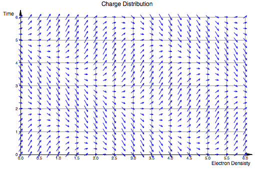
field := plot::VectorField2d([1, 3*sin(x+1+y)], x=0..6, y=0..6, Mesh=[25,25]):
plot(field, Header = "Charge Distribution", AxesTitles = ["Electron Densisty", "Time"], GridVisible = TRUE)
plot(field, Header = "Charge Distribution", AxesTitles = ["Electron Densisty", "Time"], GridVisible = TRUE)
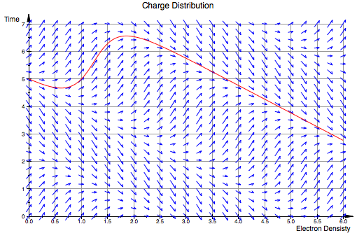
Finally, if you want to super-impose a solution line onto your plot, here is the next block of code:
f := (x, y) -> [(function)]:
solution1 := numeric::odesolve2(f, initialx, [initialy]):
curve1 := plot::Function2d(solution1(x)[1], x = start .. end, LineColor = RGB::Red):
plot(field, curve1, GridVisible = TRUE)
solution1 := numeric::odesolve2(f, initialx, [initialy]):
curve1 := plot::Function2d(solution1(x)[1], x = start .. end, LineColor = RGB::Red):
plot(field, curve1, GridVisible = TRUE)
First we map F as a function. For "function" you need to place a [1] next to any "y" variable. For example [(x^2 + 2*y[1])]. Next we solve numerically using the odesolve2 function. "initialx" and "[initially]" should be your intial value such that f(initial) = initial(y). These should be real numbers. Next we define our curve as the plot of this solution, given a starting and ending point (usually the same start/end as before). I like to make the line color red so it pops out. Then, as before, we plot our field function as well as the curve function this time, on the same graph. Below is a full example.
field := plot::VectorField2d([1, 3*sin(x+1+y)], x=0..6, y=0..7, Mesh=[25,25]):
f := (x, y) -> [3*sin(x+1+y[1])]:
solution1 := numeric::odesolve2(f, 0, [5]):
curve1 := plot::Function2d(solution1(x)[1], x=0..6, LineColor = RGB::Red):
plot(field, curve1, Header = "Charge Distribution", AxesTitles = ["Electron Densisty", "Time"], GridVisible = TRUE)
f := (x, y) -> [3*sin(x+1+y[1])]:
solution1 := numeric::odesolve2(f, 0, [5]):
curve1 := plot::Function2d(solution1(x)[1], x=0..6, LineColor = RGB::Red):
plot(field, curve1, Header = "Charge Distribution", AxesTitles = ["Electron Densisty", "Time"], GridVisible = TRUE)
Home |
< Previous |
Next > |