Examples

Throwing a Ball

Consider a problem of throwing a ball in vertical direction with some initial velocity. It is known from elementary physics that, in the absence of air friction, a ball thrown up from the ground into earth's atmosphere with initial speed $v_0$ would attain a maximum altitude of $v_0^2 /(2g)$. In this case the return time is $2\, v_0 /g$, independent of the ball's mass. Here $g$ is the acceleration due to gravity. If the ball is thrown up from altitude $y_0$ (which we later assume to be zero), then the time $T_0$ spent traveling is given by

T_0 = (v_0 + sqrt(v_0^2 + 2 y_0 g))/g

The presence of air influences the ball's motion: it experiences two forces acting on it---the force of gravity and the air resistance force. Let's define the symbol $T$ as follows

T is travel time with air resistance when thrown from height $y_0$

Without air resistance, the object travels farther up than with air resistance. On the way down, without air resistance the object travels a larger distance, but it also gathers more speed. A natural question is, which travel time (with air resistance vs. no air resistance) is larger? Also, it is of interest to find the maximum altitude $y_{\max}$ of the ball, the time $T_{\max}$ to reach maximum altitude, and the time $T_{\text{down}}$ to return back from $y_{\max}$. Therefore,
$T_{max} + T_{down} = T_{total}$
(the total time the ball spent in the air). The landing velocity is denoted by $v_{land}$.

Air resistance is the force that acts in the direction opposite to the motion of an object through air. Air resistance depends on the shape, material, and orientation of the object, the density of the air, and the object's relative speed. We would like to think that there is a nice formula for the air resistance in terms of speed and other variables. Such a formula would help in making alculations and predicting various quantities. A starting point for obtaining such a formula is our everyday experience.

Based on our experience, a reasonable assumption to make is that air resistance increases in magnitude as a function of speed,

and that there is no air resistance if the object has speed zero. Our intuition based on everyday experience is limited to a small range of conditions. This may lead to erroneous assumptions. It has been observed that, under suitable conditions, the magnitude of the air resistance is proportional to a power of the speed $s=|v|$:

 

F ~ s^p <=> F(v) = k |v|^p .

 

Here $v$ is velocity, and both $k$ and $p$ are positive constants. For very small objects, such as a speck of dust (about 1 micrometer or 0.001mm), $p=1$ seems to give a reasonable formula for the air resistance. For larger, human scale objects moving at relatively large speed, $p=2$ works better.

 

Defining the constants:

Calculating the left-hand side of the equation that gives us the landing velocity, here denoted by x:

Calculating the right-hand side of the equation that gives us the landing velocity:

Solving for the landing velocity

out= {-26.53343153, 26.53343153}

Ascribing only the negative solution that makes sense to a new variable landing_velocity:

out= -26.53343153

The total time it takes the object to fall down to the initial height. This calculation verifies the respective value provided to us in the handout:

out= 7.215794318
The total time it takes the object to fall down to the initial height if there was no air pressure:
out= 10.20408163

Ratio between Ttotal and T0. This calculation verifies the respective value provided to us in the handout:

out= 0.7071478431

Example (contuniation)

 

out= -4.919081053
out= 9.647612103
out= 2.003349654
out= 2.039567612
out= y=0.9822423355

 

out= -4.919081053

Calculating the left-hand side of the equation that gives us the landing velocity, where the initial velocity is denoted by y:

Calculating the right-hand side of the equation that gives us the landing velocity, denoted here by x:

Plotting the landing velocity versus the initial velocity in the v0 interval [0; 10]:

Solving for the landing velocity in terms of the initial velocity:

Solving for the total time it takes for the object to fall down to its initial height:

Plotting the total time, Ttotal, versus initial velocity, for the v0 interval [0; 10]:

 

Example (contuniation)

Defining the constants:

Finding Tmax using the formula provided in Part 6 of the handout:

out= 0.95842211

Solving for landing velocity vl using Equation (1) from the handout:
1) Evaluating the left-hand side:

2) Evaluating the right-hand side:

out= -4.642928642

3) Solving for the unknown variable: the landing velocity:

out= {-9.113223762, 9.113223762}

4) Since the landing velocity has to have a negative value:

out= -9.113223762

Ultimately, we can find Tdown using the formula for T - Tmax, provided in Part 6 of the handout:

out= 0.988547443

Notice that there are 3 basic parameters- function, independent variable window width, and dependent window width. As with most MuPad functions, the function itself comes first. Another good parameter to use is 'GridVisible = TRUE' to turn on the grid for yourself.

To plot more than one function on the same graph, you can separate them by commas as different parameters in the same plot function.

When defining a function to plot (separate from inside the plot function), sometimes it is nice to include a parameter for the line color - 'LineColor = RGB::Red' - which literally stands for 'choose between red green and blue for your line'.
Notice that there is an extra identifier in front of the plot function this time '::Function2d'. This is just to indicate to MuPad that we want it to be a 2 dimensional graph in cases of a 3 dimensional object. In the case where you are plotting objects of multiple variables, this can be very useful. To get a 3 dimensional graph, all you have to do is change the '2' above to a '3'.

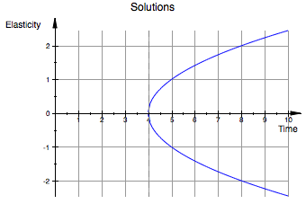
Labels are used as parameters inside the plot function. The syntax is as follows: 'Header = ['This Is My Title']' and 'AxesTitles = ['Xaxis Title', 'YAxis Title']'. Here is an example with all the aspects at once: