Integrating FactorsBrown University, Applied Mathematics |
Integrating factors
Find an integrating factor \( \mu = \mu (y) \) that makes the following equation exact. First we solve the equation:
pO6 := ode((4*y(x)^2+1/2*x*y(x))-3*x^3*diff(y(x),x)=0, y(x))
solve(O6)
solve(O6)
Find an integrating factor \( \mu = \mu (x) \) that makes the following equation exact. First we solve the equation:
O7:= ode((3*y(x)*x+y(x)^2)+(x^2+x*y(x))*diff(y(x),x)=0,y(x))
solve(O7)
solve(O7)
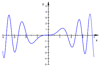
To plot more than one function on the same graph, you can separate them by commas as different parameters in the same plot function.
plot(function1, function2, x=start..end, y=start..end)
When defining a function to plot (separate from inside the plot function), sometimes it is nice to include a parameter for the line color - 'LineColor = RGB::Red' - which literally stands for 'choose between red green and blue for your line'.
curve1 := plot::Function2d(function3,t=0..10, LineColor = RGB::Red)
Notice that there is an extra identifier in front of the plot function this time '::Function2d'. This is just to indicate to MuPad that we want it to be a 2 dimensional graph in cases of a 3 dimensional object. In the case where you are plotting objects of multiple variables, this can be very useful. To get a 3 dimensional graph, all you have to do is change the '2' above to a '3'.
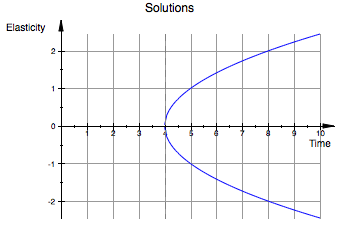
Labels are used as parameters inside the plot function. The syntax is as follows: 'Header = ['This Is My Title']' and 'AxesTitles = ['Xaxis Title', 'YAxis Title']'. Here is an example with all the aspects at once:
curve1 := (sqrt(x -4),LineColor = RGB::Blue)
curve2 := (-sqrt(x -4))
plot(curve1,curve2, x=0..10, y=-5..5, Header = 'Solutions', AxesTitles = ['Time','Elasticity'],GridVisible = TRUE)
curve2 := (-sqrt(x -4))
plot(curve1,curve2, x=0..10, y=-5..5, Header = 'Solutions', AxesTitles = ['Time','Elasticity'],GridVisible = TRUE)
Home |
< Previous |
Next > |