Applications

Brown University, Applied Mathematics

Plotting Syntax

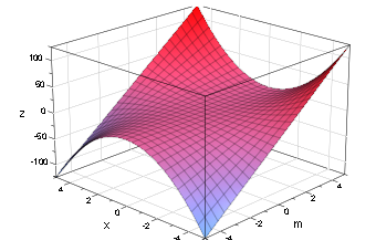
MuPAD can plot many kinds of functions for you. Different kinds of plots are denoted by the extra '::' add on after the word 'plot'. The only tricky part is that sometimes you have to call 'display(%)' right after the function so that it will actually show up. Some of these kinds of plots even include animations when you click on them! To interact with plots, double click on the image and you should be able to move around, which can be very useful for 3 dimensional plots.

Function graphs
plot::Function2d, plot::Function3d
Curves
plot::Curve2d, plot::Curve3d
Points
plot::Point2d, plot::Point3d
Lines
plot::Line2d, plot::Line3d
Polygons
plot::Polygon2d, plot::Polygon3d
Surfaces
plot::Surface
Complex objects
plot::VectorField2d, plot::Ode2d, plot::Ode3d, plot::Implicit2d, plot::Implicit3d

Useful Parameters

These are things to include at the end of your plot function, seperated by commas, and stil within the parenthesis of the plot function.

GridVisible = TRUE
turns on a grid for the plot
TicksDistance = YOURNUMBER
works if the grid is visible and allows you to manipulate the size of the grid squares where YOURNUMBER is a non-negative integer
Scaling = Constrained
forces the y-axis to have the same scale as the x-axis
CoordinateType = LinLog
forces a linear logarithmic plot
CoordinateType = LogLog
forces a logarithmic scale on both the x and y axis
#Arrows
forces the curve to be an arrow
#Legend
creates an automatic legend for you at the bottom of the plot
piecewise(...)
allows you to define a piecewise function to plot

Examples

plot(m*x^2, #3D, GridVisible=TRUE)

plot::Curve3d([sin(t), cos(t), 0.3*t], t=0..a, a=0..8*PI)

display(%)

(refresh the page to see the animation in action)

Plotting Solutions to IVPs

The beauty of Mupad is that you can plot anything using the magical command ‘display(%)’. Now to solve an initial value problem you can use the command ‘IVP := ode({“diffeqn.”, “initial value(s)”}, y(x))’. Breaking down the code: “IVP” is just the name I randomly assigned to the equation and it can be replaced with any letter. “ode” is the built-in Mupad function that solves differential equations. (In it’s sleep) “diffeqn” is the differential equation you wish to solve. “initial value(s)” are the initial conditions and “y(x)” is there for syntax purposes.

IVP := ode({y'(x)= -2*x*y(x), y(0)=1}, y(x))
solve(IVP)
display(%)

Another example

a:= ode({y''(x) = x-3, y(0) = 5, y'(0) = 1}, y(x))

plot(solve(a), x=a..b)