The Laplace TransformBrown University Applied Mathematics |
Solving Differential Equations with the Laplace Transform
We will use the derivative rule in terms of our dependent variabe "y" to create a function in terms of $y^{L}$ which we can then isolate, and then apply the Laplace Transform to. Then we will apply the Inverse Laplace transform to obtain our answer. The process is just as simple as I just layed out:
1. Use Derivative Rule
2. Isolate $y^{L}$
3. Apply Laplace Transform
4. Apply Inverse Laplace Transform
5. Make sure to multiply by the Heaviside function
The entire process can be done in MuPAD using all the commands that we know. It is important to note that our answer will be unique - we will be solving IVP/Cauchy problems. When we use the derivative rule, we end up with a place for the initial conditions, which works perfectly for us! The best way to learn this is by example - simply working through multiple problems.
Example Problems
Homogeneous, Characteristic Equation has Real Roots $y''+5y'+6y = 0$ such that $y(0)=0, y'(0)=1$
First we want to apply the derivative rule to our function:
For the y'' term we obtain:
$\lambda^2*y^{L}-y'(0)-\lambda y(0)$
For the 5y' term we obtain:
$5(\lambda y^{L}-y(0))$
And finally for the 6y term we obtain:
$6y^{L}$
reset()
assume(t>0)
homogeneous := `λ`^2*L[y]-y'(0)-`λ`*y(0)+5*(`λ`*L[y]-y(0))+6*L[y]
![]()
solve(homogeneous=0,L[y],IgnoreSpecialCases)
![]()
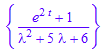
ourtransform:=subs(%,[y(0)=0,y'(0)=1])
![]()
ilaplace::addpattern(pat, s, t, res)
ilaplace(ourtransform[1],`λ`,t)
![]()
(%)*H(t)
![]()
Nonhomogeneous Continuous, Characteristic Equation has Real Roots
$y''+5y'+6y = e^2t$ such that $y(0)=0, y'(0)=1$
Again, we want to apply the derivative rule to our function:
For the y'' term we obtain:
$\lambda^2*y^{L}-y'(0)-\lambda y(0)$
For the 5y' term we obtain:
$5(\lambda y^{L}-y(0))$
And finally for the 6y term we obtain:
$6y^{L}$
reset()
assume(t>0)
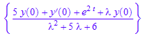
homogeneous := `λ`^2*L[y]-y'(0)-`λ`*y(0)+5*(`λ`*L[y]-y(0))+6*L[y]
![]()
forcingterm := e^(2*t)
![]()
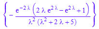
solve(homogeneous=forcingterm,L[y],IgnoreSpecialCases)
ourtransform:=subs(%,[y(0)=0,y'(0)=1])
ilaplace::addpattern(pat, s, t, res)
ilaplace(ourtransform[1],`λ`,t)
![]()
(%)*H(t)
![]()
Nonhomogeneous Continuous, Characteristic Equation has a Double Root
$y''-y = \sin(6t)$ such that $y(0)=6, y'(0)=2$
reset()
assume(t>0)
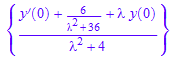
homogeneouspart := `λ`^2*L[y]-y'(0)-`λ`*y(0)-L[y]
![]()
forcingterm := laplace(sin(6*t),t,`λ`)
![]()
solve(homogeneouspart=forcingterm,L[y],IgnoreSpecialCases)
ourtransform := subs(%,[y(0)=6, y'(0)=2])
ilaplace::addpattern(pat, s, t, res)
ilaplace(ourtransform[1],`λ`,t)
![]()
%*H(t)
![]()
Nonhomogeneous Continuous, Characteristic Equation has Complex Roots
$y''+4y = \sin(6t)$ such that $y(0)=6, y'(0)=2$
reset()
assume(t>0)
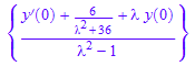
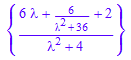
homogeneouspart := `λ`^2*L[y]-y'(0)-`λ`*y(0)+4*L[y]
![]()
forcingterm := laplace(sin(6*t),t,`λ`)
![]()
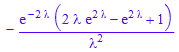
solve(homogeneouspart=forcingterm,L[y],IgnoreSpecialCases)
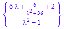
ourtransform := subs(%,[y(0)=6, y'(0)=2])
ilaplace::addpattern(pat, s, t, res)
ilaplace(ourtransform[1],`λ`,t)
![]()
%*H(t)
![]()
Nonhomogeneous Piecewise Continuous, Characteristic Equation has Complex Roots
$y''+2y'+5y = = \begin{cases} t-2 &\mbox{if } 0 \leq t \leq 2 \\0 &\mbox{if } 2 \leq t \\ \end{cases}$ such that $y(0)=0, y'(0)=0$
reset()
assume(t>0)
homogeneouspart := `λ`^2*L[y]-y'(0)-`λ`*y(0)+2*(`λ`*L[y]-y(0))+5*L[y]
![]()
f := simplify((t-2)*(heaviside(t)-heaviside(t-2)))
![]()
laplace::addpattern(pat, t, s, res)
forcingterm := laplace(f,t,`λ`)
solve(homogeneouspart=forcingterm,L[y],IgnoreSpecialCases)
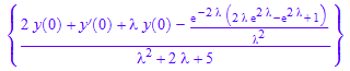
ourtransform := subs(%,[y(0)=0, y'(0)=0])
ilaplace::addpattern(pat, s, t, res)
ilaplace(ourtransform[1],`λ`,t)

%*H(t)

Home |
< Previous |
Next > |