A simple pendulum consists of a single point of mass m (bob) attached
to a rod (or wire) of length \( \ell \) and of
negligible weight. We denote by θ the angle measured between the
rod and the vertical axis, which is assumed to be positive in
counterclockwise direction. By applying the Newton’s law of dynamics, we obtain the equation of motion
It can be simplified by putting \( \omega = \sqrt{g/\ell} : \)
\[
\ddot{\theta} + \omega^2 \sin \theta =0 .
\]
Further simplification is available by normalization, which leads to \( \omega = 1 \) and we get
\[
\ddot{\theta} + \sin \theta =0 .
\]
In practice, it is easier to study an ordinary differential equation as a system of equations involving only the first derivatives.
\[
\dot{x} = y, \qquad \dot{y} = -\sin x .
\]
The variables x and y can be interpreted geometrically. Indeed, the angle x = θ corresponds to a point on a circle whereas the velocity \( y = \dot{\theta} \) corresponds to a point on a real line. Therefore, the set of all states (x ,y) can be represented by a cylinder, the product of a circle by a line. More formally, the phase space of the pendulum is the cylinder \( S^1 \times \mathbb{R} , \) its elements are couples (position,velocity).
Thus, at each point (x ,y) in the phase space, there is an attached vector
\( (\dot{x}, \dot{y} ) = (y, - \sin x) . \) This can be geometrically represented as a
vector field on the cylindrical phase space.
Example: Consider the matrix
You can draw phase portrait for the pendulum not on the plane \( \mathbb{R}^2 , \) but
on the cylinder \( S^1 \times \mathbb{R} . \) The pendulum of course has only two
equilibria, one at (0,0) and another one at (π,0).
The vector field can also be interpreted as a velocity vector field. This means that a point x in the phase space moves along a trajectory so that its velocity vector at each instant equals the vector of the vector field attached to the location of x. Such a trajectory X(t), also called an orbit, trajectory, streamline, is simply the solution of an ordinary differential equation
\[
\dot{\bf x} = {\bf f}({\bf x}) ,
\]
where f is the vector field defined by \( {\bf f} ({\bf x}) = (y, -\sin x ) . \) It is however more convenient to represent the trajectories on a plane instead of on a cylinder. This can be done by expanding the cylindrical phase space by periodicity onto a phase plane. The following diagram is called a phase portrait.
The length of the pendulum is increasing by the stretching of the wire due to the weight of the bob. The effective
spring constant for a wire of rest length \( \ell_0 \) is
\[
k = ES/ \ell_0 ,
\]
where the elastic modulus (Young's modulus) for steel is about
\( E \approx 2.0 \times 10^{11} \)
Pa and S is the cross-sectional area. With pendulum 3 m long,
the static increase in elongation is about
\( \Delta \ell = 1.6 \) mm, which is clearly not negligible. There is also dynamic
stretching of the wire from the apparent centrifugal and Coriolis forces acting on the bob during motion. We can
evaluate this effect by adapting a spring-pendulum system analysis. We go from rectangular to polar coordinates:
where \( z_0 = \ell_0 + mg/k \) is the static pendulum length,
\( \ell = z_0 \left( 1 + \xi \right) \) is the dynamic length, ξ is the fractional
string extension, and θ is the deflection angle. The equations of motion for small deflections are
where the overdots denote differentiation with respect to time t, \( \omega_p^2 = g/z_0 \)
is the square of the pendulum frequency, and \( \omega_s^2 = k/m \) is the spring
(string) frequency, squared.
To get a feeling for how rigid and massive the pendulum support must be, we model the support as mass M
kept in place by a spring of constant K, as shown in the picture below.
where x is the displacement of the rigid support. The former equation says that the effect of sway is to
impart an additional angular acceleration \( - \ddot{x}/\ell \) to the pendulum
for small angles of oscillation (otherwise, we have to use \( \omega_0^2 \sin \theta \)
instead of \( \omega_0^2 \theta \) ).
Here \( \gamma = c/(m\,\ell ) , \ \omega^2 = g/\ell \) are positive constants. Therefore, the above system of differential equations is autonomous. Setting \( \gamma = 0.25 \quad\mbox{and}\quad \omega^2 =1 , \) we ask Mathematica to provide a phase portrait for the pendulum equation with resistance:
Then, we define a routine which gives the result of integrating the differential
equation with NDSolve, starting at t = 0, and integrating out to t = tfinal.
The output sol1 contains the two interpolating functions (Mathematica uses cubic splines) that represent x(t) and v(t). We can evaluate them or plot
them. For example, the values at t = 3 are
sol1 /. t -> 3
Out[11]= {-0.6186, -0.201005}
We now plot x and v as functions of t, using solid for x and dashed for v.
For this underdamped oscillator, we see that the phase plot is a spiral. As time increases, the system point moves inward towards the equilibrium at x = 0, v = 0. In physical terms, the oscillations decrease in amplitude as the damping takes energy out of the system.
We could also construct the plot without referring separately to sol1 contains the two interpolating functions (Mathematica uses cubic splines) that represent x(t) and v(t). We can evaluate them or plot
them. For example, the values at t = 3 are
sol1 /. t -> 3
Out[11]= {-0.6186, -0.201005}
We now plot x and v as functions of t, using solid for x and dashed for v.
For this underdamped oscillator, we see that the phase plot is a spiral. As time increases, the system point moves inward towards the equilibrium at x = 0, v = 0. In physical terms, the oscillations decrease in amplitude as the damping takes energy out of the system.
We could also construct the plot without referring separately to xsol1 and ysol1.
Every solution of this equation spirals in toward the equilibrium point at {0,0}. None of these spirals intersect other
spirals, and none intersects itself. The phase plane provides an excellent way to visualize such a family of solutions. If we
attempt to view these solutions simultaneously as functions of t, the result is quite cluttered:
Planar oscillations of elastic (spring) pendulum was first considered by
Vitt, A. (Aleksandr Adolʹfovich) and Gorelik, G. (Gabriel Simonovich) in 1933.
Its translation from the Russian in English by Lisa Shields with an
introduction by Peter Lynch is available on the web.
The three dimensional spring pendulum was considered by
P. Pokorny in 2008.
The problem investigated by Vitt & Gorelik has only two degrees of freedom, namely the vertical and one
of the horizontal dimensions. According to Gabriel Gorelik, the study was motivated by the Russian physicist L. I. Mandelshtam,
who suggested this research topic as a worthy analogue of the recurrence phenomenon in the infrared spectrum of
CO2, which is known today as Fermi resonance.
Of particular interest is the case where the frequency of the vertical motion is exactly or nearly twice the frequency
of the horizontal. Under those circumstances the vertical oscillations become parametrically unstable, and any
small initial deviation of the bob from the vertical line through the spring support results in exponentially
increasing horizontal (or pendulum) oscillation. The growth of the latter stops eventually, as most of the energy of
the original vertical oscillations is converted into energy of pendulum motion. The process is now reversed as the
centrifugal force, with two cycles of oscillation in the pendulum period, acts as a forcing or excitation term to the
vertical harmonic oscillations. This phenomenon is a called parametric
resonance of the coupled system, which manifests itself as an energy transfer from one component to the other
and vice versa. The speed and amplitude of the energy transfer depend essentially on the initial conditions.
The elastic pendulum has been analyzed previously, either as a mechanical problem, or in conjunction with other
parametric phenomena, such as wave-wave coupling in plasma physics and non-linear optics, and also in the problem of
the coupling of vertical and radial oscillations of particles in cyclic accelerators.
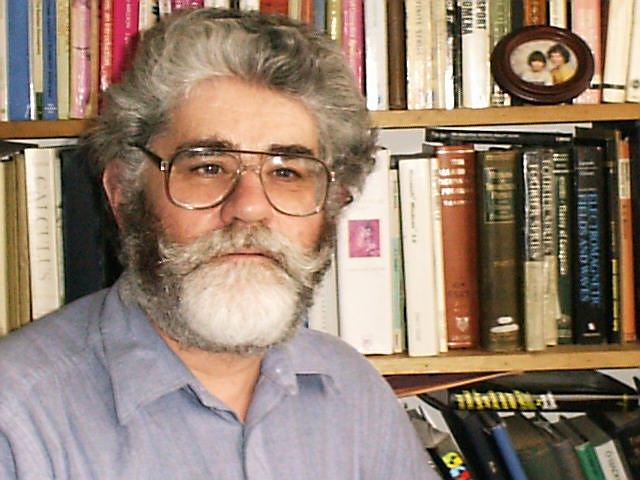
The applied mathematician, the popularizer of mathematics, research meteorologist, academic, and Irish Times columnist
Peter Lynch (Dublin) initialized a research on wide class of systems modeled by an integrable approximation to
the 3 degrees of freedom elastic pendulum with 1:1:2 resonance, or the swing-spring.
He explained the phenomenon of the splitting of the spectral lines in the CO2 molecule
(Raman scattering).
This simple system under study possesses a rich and varied range of dynamical behavior. It has many analogues in
other areas. For example, electrical systems with two degrees of freedom can be treated in similar ways, e.g., two
oscillating circuits coupled by a transformer with an iron core.
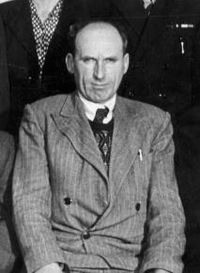
Gabriel Gorelik was born into a Jewish family in Paris in 1909. He later studied theoretical physics under Mandelstam in Lomonosov Moscow State University, and then worked under A.A. Andronov, where he was later bullied in 1952 for his "ideological mistakes," as were many others at the time. Gorelik was tragically killed by a train in 1956.
Gorelik's father, Simon, sacrificed his own life to save Moscow from a
pneumonic plague outbreak in 1939 by diagnosing the disease,
and then locking himself and the infected people inside the building while trying to save the life of the microbiologist Berlin, so that only twelve people died from the plague, including Simon Gorelik.
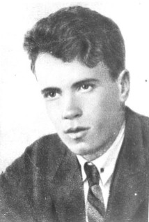
Aleksandr Adolfovich Vitt also suffered a tragic fate. Vitt was born
in Russia in 1902 to ethnic German parents, and he also studied under
Mandelstam then later Andronov. Vitt was then persecuted during the
Great Purge in 1938 and was sentenced to 5 years of labor camps where
he died soon after 1938.
Leonid Isaakovich Mandelstam, or Mandelshtam (1879--1944) was a Soviet physicist of Belarusian-Jewish background.
Leonid Mandelstam was born in Mogilev, Russian Empire (now Belarus). He studied at the Novorossiya University in
Odessa, but was expelled in 1899 due to political activities, and continued his studies at the University of
Strasbourg. He remained in Strasbourg until 1914, and returned with the beginning of World War I. He was awarded
the Stalin Prize in 1942. Mandelstam died in Moscow, USSR (now Russia). He was a co-discoverer of inelastic
combinatorial scattering of light used now in Raman spectroscopy.
In 1918, Mandelstam theoretically predicted the fine structure splitting in
Rayleigh scattering
due to light scattering on thermal acoustic waves. Beginning from
1926, L.I. Mandelstam and G.S. Landsberg initiated experimental
studies on vibrational scattering of light
in crystals at the Moscow State University. As
a result of this research, Landsberg and Mandelstam discovered the
effect of the combinatorial scattering of light on 21 February
1928. They presented this fundamental discovery for the first time at
a colloquium on 27 April 1928. They published brief reports about this
discovery (experimental results with theoretical explanation) in
Russian and in German, then they published a comprehensive paper in Zeitschrift fur Physik.
Current interest in the swinging spring arises from the rich variety of its solutions. The swinging and springing
oscillations act as analogues of the Rossby and gravity waves in
the atmosphere and may provide the basis for a paradigm of the most important interannual variation in
the ocean-atmosphere climate system.
For very small amplitudes, the motion is regular.
As the amplitude is increased, the regular motion breaks down into a chaotic regime that
occupies more and more of phase space as the energy grows. However, for very large energies, a regular and
predictable regime is re-established (Núñez-Yépez, H N, A L Salas-Brito, C A Vargas and L Vicente, 1990:
Onset of chaos in an extensible pendulum. Phys. Lett., A145, 101-105). This can easily be
understood: for very high energies, the system rotates rapidly around the point of suspension and is no longer vibratory.
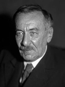
Nicolas Minorsky
The elastic pendulum problem became well known to the public after publication in 1947 of the famous book
"Introduction to Non-Linear Mechanics" by Nicolas
Minorsky (1885--1970). Nikolai Fyodorovich Minorsky was a Russian
American control theory mathematician, engineer, and applied scientist. He is best known for his theoretical analysis
and first proposed application of PID controllers in the automatic steering systems for U.S. Navy ships. He was
educated at the Nikolaev Maritime Academy in St. Petersburg (Russia), and at the University of Nancy (France).
For a year in 1917 to 1918 he was the adjunct Naval Attache at the Russian Embassy to France in Paris. In the midst
of the Russian civil war Minorsky emigrated to the United States in June 1918.
From 1924–1934 Nicolas Minorsky was a Professor of Electronics and Applied Physics at the University of Pennsylvania.
He received his PhD in physics from Penn in 1929. Minorsky worked on roll stabilization of ships for the Navy from
1934 to 1940, designing in 1938 an activated-tank stabilization system into a 5-ton model ship. His work was used for
stabilizing of aircraft carriers during the landing of airplanes.
Our exposition of elastic pendulum follows the Minorsky's book. Let us consider a massless spring of rest length
\( \ell_0 \) hung with a bob of mass m on its lower end; also let r be
its length under load, k the spring constant, and g the acceleration of
gravity. We assume that the pendulum is constrained to move in a fixed vertical plane, with the origin at the pivot
when Cartesian coordinates or polar coordinates are employed. Obviously the system possesses two degrees of freedom,
namely, the angle θ of the pendulum and
the elongation r of the spring.
Let \( \ell = \ell_0 + \frac{mg}{k} \) be the length of the spring at equilibrium when
the bob is attached because \( k \left( \ell - \ell_0 \right) = mg , \) where k is
the spring constant in Hooke's law. The deviation from the loaded equilibrium is described in rectangular coordinates as
where \( r^2 = \left( \ell -y \right)^2 + x^2 . \)
The first term of the potential energy corresponds to the elasticity of
the suspension and the second to gravity. Their derivatives are
The spring-mass oscillator is generally presumed to be one of the
simplest and most basic physical systems. In the previous section,
we considered massless spring with attached bob of mass m. Because a real spring has a finite distributed mass,
we consider the bob that is suspended on a
homogeneous elastic spring of mass ms with the elasticity constant k. Our exposition of
this problem follows closely Pavel Pokorny's article
Denoting the rectangular coordinates of the bob by X, Y, and Z, and assuming the
spring is stretched homogeneously, the kinetic energy of the system consisting of the spring with the bob becomes
are squares of frequencies for the pendulum (or quasi-horizontal) motion and the spring (or vertical) motion, respectively.
Note that p > 0 is equivalent to 0 < γ < 1, which means that \( \omega_p
< \omega_s . \)
A double pendulum consists of one pendulum attached to another. Double pendula are an example of a simple physical
system which can exhibit chaotic behavior with a strong sensitivity to
initial conditions. Several variants of the double pendulum may be considered. The two limbs may be of equal or unequal lengths and masses; they may be simple pendulums/pendula or compound pendulums (also called complex pendulums) and the motion may be in three dimensions or restricted to the vertical plane.
Consider a double bob pendulum with masses m1 and
m2, attached by rigid massless wires of lengths \( \ell_1 \) and
\( \ell_2 . \)
Further, let the angles the two wires make with the vertical be denoted
\( \theta_1 \) and
\( \theta_2 , \) as illustrated at the
left.
Let the origin of the Cartesian coordinate system is taken to be at
the point of suspension of the first pendulum, with vertical axis
pointed up.
Finally, let gravity be given by g.
Then the positions of the bobs are given by
Vitt, A. (Aleksandr Adolʹfovich) and Gorelik, G. (Gabriel Simonovich), Oscillations of an Elastic Pendulum as an Example of the Oscillations of Two
Parametrically Coupled Linear Systems,
Journal of Technical Physics, 1933, vol. 3, pp. 294–307.
Its translation from the Russian in English by
Lisa Shields with an introduction by Peter Lynch is available on the web:
http://copac.jisc.ac.uk/id/15694518?style=html
http://catalogue.nli.ie/Record/vtls000058645