Preface
This tutorial is an introduction to the programming package Matlab (created by MathWorks© ). This is a tutorial made solely for the purpose of education. The tutorial accompanies the textbook Applied Differential Equations. The Primary Course by Vladimir Dobrushkin, CRC Press, 2015; http://www.crcpress.com/product/isbn/9781439851043.
If you have not taken or are not taking a course regarding Matlab or programming, such as CSCI 0150 or ENGN 0030, then please start with Tutorial for the first course. Otherwise, please begin from Part 1 of the first course, where you should learn how to define functions and solutions to ODEs. For those who have used Matlab before, please note that there are certain commands and sequences of input that are specific for solving differential equations, so it is best to read through this tutorial in its entirety. MathWorks updates Matlab every year. Therefore, tutorials from other sources may or may not be compatible with this tutorial.
This tutorial corresponds to the Matlab “m” files that are posted on the APMA 0340 website. You, as the user, are free to use the m files to your needs for learning how to use the Matlab program, and have the right to distribute this tutorial and refer to this tutorial as long as this tutorial is accredited appropriately. Any comments and/or contributions for this tutorial are welcome; you can send your remarks to <Vladimir_Dobrushkin@brown.edu>
Return to computing page for the first course APMA0330
Return to computing page for the second course APMA0340
Return to Matlab tutorial page for the first course (APMA0330)
Return to the main page for the course APMA0340
Return to the main page for the course APMA0330
1. 3D plotting
Matlab provides many useful instructions for the visualization of 3D data. The instructions provided include tools to plot wire-frame objects, 3D plots, curves, surfaces, etc. and can automatically generate contours, display volumetric data, interpolate shading colors and even display non-Matlab made images.
| Order | Function |
| plot3(x,y,z,'line shape') | Space curve |
| meshgrid(x,y) | Mesh plot |
| mesh(x,y,z) | hollow mesh surface |
| surf(x,y,z) | mesh surface, solid filled |
| shading flat | flat/smooth surface space |
| countour3(x,y,z,n) | 3-dimensional equivipotential (n) lines |
| contour(x,y,z) | contours |
| meshc(x,y,z) | hollow grid graph projected by equivipotential lines |
| [x,y,z]=cylinder(r,n) | 3-dimensional curve surfaces |
We show how to use plotting commands by examples.
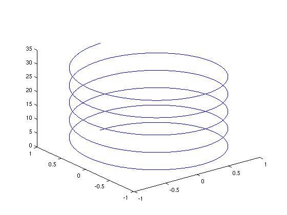
Example 0.1.1:
In the interval [0, 10*pi], draw the parametric curve:
x = sin(t), y = cos(t), z = t .
>> t=0:0.01:10*pi;
>> plot3(sin(t),cos(t),t)
Example 0.1.2:
Plot a surface z=(x+y)^2
>> x=-3:0.1:3;
>> y=1:0.1:5;
>> [x,y]=meshgrid(x,y);
>> z=(x+y).^2;
>> plot3(x,y,z)
When using ``meshgrid,'' the coding should be changed into:
>> x=-3:0.1:3;
>> y=1:0.1:5;
>> [x,y]=meshgrid(x,y);
>> z=(x+y).^2;
>> mesh(x,y,z)

Or the solid filled:
>> x=-3:0.1:3;>> y=1:0.1:5;
>> [x,y]=meshgrid(x,y);
>> z=(x+y).^2;
>> surf(x,y,z)

And with the flat surface:
>> x=-3:0.1:3;
>>
y=1:0.1:5;
>>
[x,y]=meshgrid(x,y);
>>
z=(x+y).^2;
>>
surf(x,y,z)
>>
shading flat
Example 0.1.3:
Consider a 3-dimensional rotating surface ([x,y,z]=cylinder(r,n))
We plot the 3D graph for r(t)=2+sin(t)
Using “mesh, cylinder” the code will be as follows
t=0:pi/10:2*pi;
r=2+sin(t);
[x,y,z]=cylinder(r,30);
mesh(x,y,z)
with the Solid filled
t=0:pi/10:2*pi;
r=2+sin(t);
[x,y,z]=cylinder(r,30);
surf(x,y,z)
Or with the “shading flat”:
t=0:pi/10:2*pi;
r=2+sin(t);
[x,y,z]=cylinder(r,30);
surf(x,y,z)
shading flat
Example 0.1.4:
Plot the function of r(t)=2+sin(t), using the 3-dimension equipotential lines
t=0:pi/10:2*pi;
r=2+sin(t);
[x,y,z]=cylinder(r,30);
contour3(x,y,z,20)
Or:
t=0:pi/10:2*pi;
r=2+sin(t);
[x,y,z]=cylinder(r,30);
meshc(x,y,z)
Or:
t=0:pi/10:2*pi;
r=2+sin(t);
[x,y,z]=cylinder(r,30);
surfc(x,y,z)
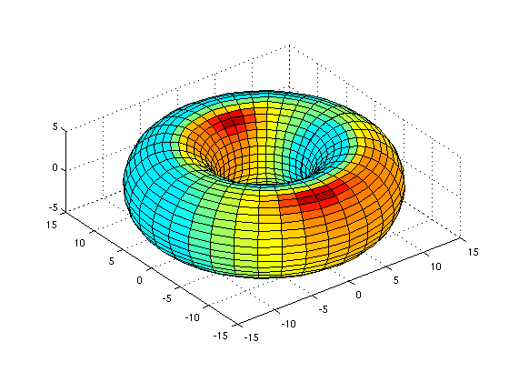
Example 0.1.5:
Toroid surface:
a=5; % a and c are arbitrary constants
c=10;
[u,v]=meshgrid(0:10:360); % meshgrid produces a full grid represented by the output coordinate arrays u and v; u and v are time variables
x=(c+a*cosd(v)).*cosd(u); % x, y, and z are the parameterized equations for a toroid
y=(c+a*cosd(v)).*sind(u);
z=a*sind(v);
surfl(x,y,z) % surfl creates a surface plot with colormap-based lighting
axis equal; % scales the axis so the x, y, and z axis are equal
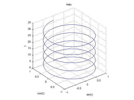
Example 0.1.4: Helix
t = 0:pi/50:10*pi; %create the vector t. starting value of 0, each element increases pi/50 from the previous up through 10*pi
plot3(sin(t),cos(t),t) %3D plot, coordinate (x, y, t)
title('Helix') %creates plot title
xlabel('sin(t)') %creates x label
ylabel('cos(t)') %creates y label
zlabel('t') %creates t label
grid on %dashed grids
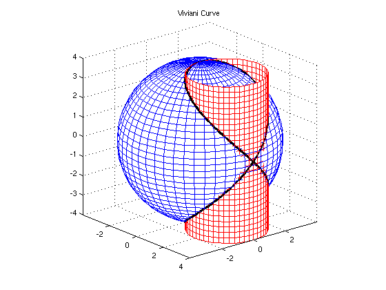
Example 0.1.5:
% The Viviani's Curve is the intersection of sphere x^2 + y^2 + z^2 = 4*a^2
%and cylinder (x-a)^2 +y^2 =a^2
%This script uses parametric equations for the Viviani's Curve,
%and the cylinder and sphere whose intersection forms the curve.
% For the sphere:
a = 2; %the parameter 'a' from the equations, here a=2
phi = linspace(0,pi,40); %this defines the scope of phi, from 0 to pi, the '40' indicates 40 increments between the bounds
theta = linspace(0,2*pi,50); %this defines the scope of theta
[phi,theta] = meshgrid(phi,theta); %creates a grid of (phi,theta) ordered pairs
%the parametric equation for the sphere:
x=2*a*sin(phi).*cos(theta); %use a '.' before the operator, this is an array operation
y=2*a*sin(phi).*sin(theta); %the . indicates that this operation goes element by element
z=2*a*cos(phi); %note: always suppress data using a semicolon
%Plotting the sphere:
mhndl1=mesh(x, y, z); %'mhndl' plots and stores a handle of the meshgrid
set(mhndl1,... % formats 'mhndl'
'EdgeColor',[0,0,1]) %gives the surface color, [0,0,1] is a color triple, vary the combination to get different color
axis equal %controls axis equality, this is very important for ensuring the sphere looks perfectly round
axis on %controls whether axes are 'on' or 'off'
%For the cylinder:
t=linspace(0,2*pi,50); %defines the scope of 't'
z=linspace(-2*a,2*a,30); %defines the scope of 'z', the bounds for the top and bottom of the cylinder
[t,z]=meshgrid(t,z); %creates pairs of (t,z)
x=a+a*cos(t); %the parametrized cylinder
y=a*sin(t);
z = 1*z;
%Plotting the cylinder
hold on %prevents override of plot data, so both the cylinder and sphere can occupy the same plot
mhndl2=mesh(x, y, z); %notice 'mhndl' is numbered, mhndl2=mesh(x,y,z) plots the cylinder
set(mhndl2,...
'EdgeColor',[1,0,0]) %[1,0,0] gives the color red
view(50,20) %view(horizontal_rotation,vertical_elevation) sets the angle of view, both parameters used are measured in degress
%For the actual Vivani's Curve:
t=linspace(0,4*pi,200); %scope of the 't' values
x= a+a*cos(t); %parametrized Viviani's Curve
y= a*sin(t);
z = 2*a*sin(t/2);
%To plot the Viviani's Curve:
vhndl = line( x,y,z); %here 'vhndl' is used to plot the curve and record the handle
set(vhndl, ...
'Color', [0,0,0],... % here [0,0,0] gives the color black
'LineWidth',3) %line width of the line
view(50,20); %similar to before, this indicates 50degrees horizontal rotation, 20 degress vertical elevation
%Adding a title
title('Viviani Curve') %to add a title, use title('Title')
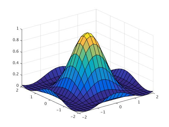
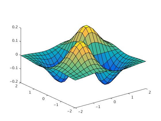
Example 0.1.6:
Some other simple 3D curves:
[x,y] = meshgrid(-2:0.2:2,-2:0.2:2);
z=x.*y.*exp(-x.^2-y.^2);
figure
surface(x,y,z)
view(3)
 z=(cos(x).^2).*(cos(y).^2);

  surf(x,y,z)