Laplace Transformation

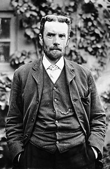
The Laplace transformation that gave birth to one of the most poweful tool in quantum mechanics---spectral decomposition method---was actually invented by British electrical engineer Oliver Heaviside (1850--1925). He was a self-taught English electrical engineer, mathematician, and physicist who adapted complex numbers to the study of electrical circuits, invented mathematical techniques for the solving linear differential equations, reformulated Maxwell's field equations in terms of electric and magnrtic forces and energy flux, and idependently co-formulated vector calculus.

The Laplace transform of a function f(t) that is defined on half line \( [0, +\infty ) \) as semi-definite integral:

\[ {\cal L} [f] (\lambda ) = f^L (\lambda ) = \int_0^{\infty} f(\lambda )\,e^{-\lambda t} \,{\text d}t . \]

Here \( \lambda \) is a parameter, which is either a complex or real number.

 

Heaviside function

The Heaviside function is a piece-wise continuous function:

\[ H(t) = \begin{cases} 1 , & \ \mbox{ if } 0 < t < \infty , \\ 1/2 , & \ \mbox{ if } t=0, \\ 0, & \ \mbox{ if } -\infty < t < 0 . \end{cases} \]

 

 

Laplace transform of discontinuous functions

If you have a piecewise-defined polynomial function then there is a “native” command for computing Laplace transforms. This calls Maxima but it’s worth noting that Maxima cannot handle (using the direct interface illustrated in the last few examples) this type of computation.

sage: var('x s')
(x, s)
sage: f1(x) = 1
sage: f2(x) = 1-x
sage: f = Piecewise([[(0,1),f1],[(1,2),f2]])
sage: f.laplace(x, s)
-e^(-s)/s + (s + 1)*e^(-2*s)/s^2 + 1/s - e^(-s)/s^2

For other “reasonable” functions, Laplace transforms can be computed using the Maxima interface:

sage: var('k, s, t')
(k, s, t)
sage: f = 1/exp(k*t)
sage: f.laplace(t,s)
1/(k + s)

is one way to compute LT’s and

sage: var('s, t')
(s, t)
sage: f = t^5*exp(t)*sin(t)
sage: L = laplace(f, t, s); L
3840*(s - 1)^5/(s^2 - 2*s + 2)^6 - 3840*(s - 1)^3/(s^2 - 2*s + 2)^5 +
720*(s - 1)/(s^2 - 2*s + 2)^4

is another way.

 

Convolution

You can find the convolution of any piecewise defined function with another (off the domain of definition, they are assumed to be zero). Here is \(f\), \(f*f\), and \(f*f*f\), where \( f(x)=1\), \(0<x<1\):

sage: x = PolynomialRing(QQ, 'x').gen()
sage: f = Piecewise([[(0,1),1*x^0]])
sage: g = f.convolution(f)
sage: h = f.convolution(g)
sage: P = f.plot(); Q = g.plot(rgbcolor=(1,1,0)); R = h.plot(rgbcolor=(0,1,1))

To view this, type show(P+Q+R).

 

Inverse Laplace transform

Numerical integration methods can prove

Residue method

Re

Differential equations

Differentiation:

sage: var('x k w')
(x, k, w)
sage: f = x^3 * e^(k*x) * sin(w*x); f
x^3*e^(k*x)*sin(w*x)
sage: f.diff(x)
w*x^3*cos(w*x)*e^(k*x) + k*x^3*e^(k*x)*sin(w*x) + 3*x^2*e^(k*x)*sin(w*x)
sage: latex(f.diff(x))
w x^{3} \cos\left(w x\right) e^{\left(k x\right)} + k x^{3} e^{\left(k x\right)} \sin\left(w x\right) + 3 \, x^{2} e^{\left(k x\right)} \sin\left(w x\right)

If you type view(f.diff(x)) another window will open up displaying the compiled output. In the notebook, you can enter

var('x k w')
f = x^3 * e^(k*x) * sin(w*x)
show(f)
show(f.diff(x))

into a cell and press shift-enter for a similar result. You can also differentiate and integrate using the commands

R = PolynomialRing(QQ,"x")
x = R.gen()
p = x^2 + 1
show(p.derivative())
show(p.integral())

in a notebook cell, or

sage: R = PolynomialRing(QQ,"x")
sage: x = R.gen()
sage: p = x^2 + 1
sage: p.derivative()
2*x
sage: p.integral()
1/3*x^3 + x

on the command line. At this point you can also type view(p.derivative()) or view(p.integral()) to open a new window with output typeset by LaTeX.

Applications

You can find critical points of a piecewise defined function:

sage: x = PolynomialRing(RationalField(), 'x').gen()
sage: f1 = x^0
sage: f2 = 1-x
sage: f3 = 2*x
sage: f4 = 10*x-x^2
sage: f = Piecewise([[(0,1),f1],[(1,2),f2],[(2,3),f3],[(3,10),f4]])
sage: f.critical_points()
[5.0]

Runge--Kutta Methods

Taylor series:

sage: var('f0 k x')
(f0, k, x)
sage: g = f0/sinh(k*x)^4
sage: g.taylor(x, 0, 3)
-62/945*f0*k^2*x^2 + 11/45*f0 - 2/3*f0/(k^2*x^2) + f0/(k^4*x^4)
sage: maxima(g).powerseries('_SAGE_VAR_x',0)    # TODO: write this without maxima
16*_SAGE_VAR_f0*('sum((2^(2*i1-1)-1)*bern(2*i1)*_SAGE_VAR_k^(2*i1-1)*_SAGE_VAR_x^(2*i1-1)/factorial(2*i1),i1,0,inf))^4

Of course, you can view the LaTeX-ed version of this using view(g.powerseries('x',0)).

The Maclaurin and power series of \(\log({\frac{\sin(x)}{x}})\):

sage: f = log(sin(x)/x)
sage: f.taylor(x, 0, 10)
-1/467775*x^10 - 1/37800*x^8 - 1/2835*x^6 - 1/180*x^4 - 1/6*x^2
sage: [bernoulli(2*i) for i in range(1,7)]
[1/6, -1/30, 1/42, -1/30, 5/66, -691/2730]
sage: maxima(f).powerseries(x,0)    # TODO: write this without maxima
'sum((-1)^i3*2^(2*i3-1)*bern(2*i3)*_SAGE_VAR_x^(2*i3)/(i3*factorial(2*i3)),i3,1,inf)

Integration

Numerical integration is discussed in Riemann and trapezoid sums for integrals below.

Sage can integrate some simple functions on its own:

sage: f = x^3
sage: f.integral(x)
1/4*x^4
sage: integral(x^3,x)
1/4*x^4
sage: f = x*sin(x^2)
sage: integral(f,x)
-1/2*cos(x^2)

Sage can also compute symbolic definite integrals involving limits.

sage: var('x, k, w')
(x, k, w)
sage: f = x^3 * e^(k*x) * sin(w*x)
sage: f.integrate(x)
((24*k^3*w - 24*k*w^3 - (k^6*w + 3*k^4*w^3 + 3*k^2*w^5 + w^7)*x^3 + 6*(k^5*w + 2*k^3*w^3 + k*w^5)*x^2 - 6*(3*k^4*w + 2*k^2*w^3 - w^5)*x)*cos(w*x)*e^(k*x) - (6*k^4 - 36*k^2*w^2 + 6*w^4 - (k^7 + 3*k^5*w^2 + 3*k^3*w^4 + k*w^6)*x^3 + 3*(k^6 + k^4*w^2 - k^2*w^4 - w^6)*x^2 - 6*(k^5 - 2*k^3*w^2 - 3*k*w^4)*x)*e^(k*x)*sin(w*x))/(k^8 + 4*k^6*w^2 + 6*k^4*w^4 + 4*k^2*w^6 + w^8)
sage: integrate(1/x^2, x, 1, infinity)
1

Convolution

You can find the convolution of any piecewise defined function with another (off the domain of definition, they are assumed to be zero). Here is \(f\), \(f*f\), and \(f*f*f\), where \(f(x)=1\), \(0<x<1\):

sage: x = PolynomialRing(QQ, 'x').gen()
sage: f = Piecewise([[(0,1),1*x^0]])
sage: g = f.convolution(f)
sage: h = f.convolution(g)
sage: P = f.plot(); Q = g.plot(rgbcolor=(1,1,0)); R = h.plot(rgbcolor=(0,1,1))

To view this, type show(P+Q+R).

Laplace transforms

If you have a piecewise-defined polynomial function then there is a “native” command for computing Laplace transforms. This calls Maxima but it’s worth noting that Maxima cannot handle (using the direct interface illustrated in the last few examples) this type of computation.

sage: var('x s')
(x, s)
sage: f1(x) = 1
sage: f2(x) = 1-x
sage: f = Piecewise([[(0,1),f1],[(1,2),f2]])
sage: f.laplace(x, s)
-e^(-s)/s + (s + 1)*e^(-2*s)/s^2 + 1/s - e^(-s)/s^2

For other “reasonable” functions, Laplace transforms can be computed using the Maxima interface:

sage: var('k, s, t')
(k, s, t)
sage: f = 1/exp(k*t)
sage: f.laplace(t,s)
1/(k + s)

is one way to compute LT’s and

sage: var('s, t')
(s, t)
sage: f = t^5*exp(t)*sin(t)
sage: L = laplace(f, t, s); L
3840*(s - 1)^5/(s^2 - 2*s + 2)^6 - 3840*(s - 1)^3/(s^2 - 2*s + 2)^5 +
720*(s - 1)/(s^2 - 2*s + 2)^4

is another way.

Ordinary differential equations

Symbolically solving ODEs can be done using Sage interface with Maxima. See

sage:desolvers?

for available commands. Numerical solution of ODEs can be done using Sage interface with Octave (an experimental package), or routines in the GSL (Gnu Scientific Library).

An example, how to solve ODE’s symbolically in Sage using the Maxima interface (do not type the ...):

sage: y=function('y',x); desolve(diff(y,x,2) + 3*x == y, dvar = y, ics = [1,1,1])
3*x - 2*e^(x - 1)
sage: desolve(diff(y,x,2) + 3*x == y, dvar = y)
_K2*e^(-x) + _K1*e^x + 3*x
sage: desolve(diff(y,x) + 3*x == y, dvar = y)
(3*(x + 1)*e^(-x) + _C)*e^x
sage: desolve(diff(y,x) + 3*x == y, dvar = y, ics = [1,1]).expand()
3*x - 5*e^(x - 1) + 3

sage: f=function('f',x); desolve_laplace(diff(f,x,2) == 2*diff(f,x)-f, dvar = f, ics = [0,1,2])
x*e^x + e^x

sage: desolve_laplace(diff(f,x,2) == 2*diff(f,x)-f, dvar = f)
-x*e^x*f(0) + x*e^x*D[0](f)(0) + e^x*f(0)

If you have Octave and gnuplot installed,

sage: octave.de_system_plot(['x+y','x-y'], [1,-1], [0,2]) # optional - octave

yields the two plots \((t,x(t)), (t,y(t))\) on the same graph (the \(t\)-axis is the horizonal axis) of the system of ODEs

\[x' = x+y, x(0) = 1; y' = x-y, y(0) = -1,\]

for \(0 <= t <= 2\). The same result can be obtained by using desolve_system_rk4:

sage: x, y, t = var('x y t')
sage: P=desolve_system_rk4([x+y, x-y], [x,y], ics=[0,1,-1], ivar=t, end_points=2)
sage: p1 = list_plot([[i,j] for i,j,k in P], plotjoined=True)
sage: p2 = list_plot([[i,k] for i,j,k in P], plotjoined=True, color='red')
sage: p1+p2
Graphics object consisting of 2 graphics primitives

Another way this system can be solved is to use the command desolve_system.

sage: t=var('t'); x=function('x',t); y=function('y',t)
sage: des = [diff(x,t) == x+y, diff(y,t) == x-y]
sage: desolve_system(des, [x,y], ics = [0, 1, -1])
[x(t) == cosh(sqrt(2)*t), y(t) == sqrt(2)*sinh(sqrt(2)*t) - cosh(sqrt(2)*t)]

The output of this command is not a pair of functions.

Finally, can solve linear DEs using power series:

sage: R.<t> = PowerSeriesRing(QQ, default_prec=10)
sage: a = 2 - 3*t + 4*t^2 + O(t^10)
sage: b = 3 - 4*t^2 + O(t^7)
sage: f = a.solve_linear_de(prec=5, b=b, f0=3/5)
sage: f
3/5 + 21/5*t + 33/10*t^2 - 38/15*t^3 + 11/24*t^4 + O(t^5)
sage: f.derivative() - a*f - b
O(t^4)

Fourier series of periodic functions

If \(f(x)\) is a piecewise-defined polynomial function on \(-L<x<L\) then the Fourier series

\[f(x) \sim \frac{a_0}{2} + \sum_{n=1}^\infty \left[a_n\cos\left(\frac{n\pi x}{L}\right) + b_n\sin\left(\frac{n\pi x}{L}\right)\right]\]

converges. In addition to computing the coefficients \(a_n,b_n\), it will also compute the partial sums (as a string), plot the partial sums (as a function of \( x\) over \((-L,L)\), for comparison with the plot of \( f(x)\) itself), compute the value of the FS at a point, and similar computations for the cosine series (if \( f(x)\) is even) and the sine series (if \(f(x)\) is odd). Also, it will plot the partial F.S. Cesaro mean sums (a “smoother” partial sum illustrating how the Gibbs phenomenon is mollified).

sage: f1 = lambda x: -1
sage: f2 = lambda x: 2
sage: f = Piecewise([[(0,pi/2),f1],[(pi/2,pi),f2]])
sage: f.fourier_series_cosine_coefficient(5,pi)
-3/5/pi
sage: f.fourier_series_sine_coefficient(2,pi)
-3/pi
sage: f.fourier_series_partial_sum(3,pi)
-3*cos(x)/pi - 3*sin(2*x)/pi + sin(x)/pi + 1/4

Type show(f.plot_fourier_series_partial_sum(15,pi,-5,5)) and show(f.plot_fourier_series_partial_sum_cesaro(15,pi,-5,5)) (and be patient) to view the partial sums.